Voronoi: Nodes and Geometry, Integrators

Nodes

The most basic thing is the creation of a list of Points. We advise to use the following:

HighVoronoi.VoronoiNodes — Method

VoronoiNodes(x::Matrix)

also available in the forms

VoronoiNodes(x::Vector{<:Vector})
VoronoiNodes(x::Vector{<:SVector})

creates a list of points (as static vectors) from a matrix.

Example: 100 Points in $(0,1)^3$

data = rand(3,100)
points = VoronoiNodes(data)

An advanced method is given by the following

VoronoiNodes(number_of_nodes::Int;density , 
            domain::Boundary=Boundary(), bounding_box::Boundary=Boundary(),
            criterium=x->true)

When density = x->f(x) this will create a cloud of approximately number_of_nodes points inside the intersection of domain and bounding_box with spatial distribution $f(x)$. Note that both exact number and position of points are random. The variable bounding_box allows to handle also the case when domain is unbounded. The intersection of domain and bounding_box HAS TO BE bounded!

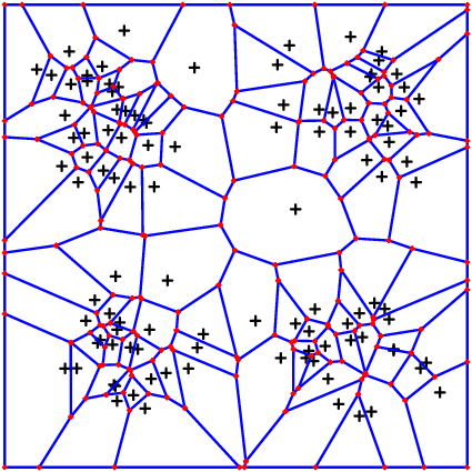
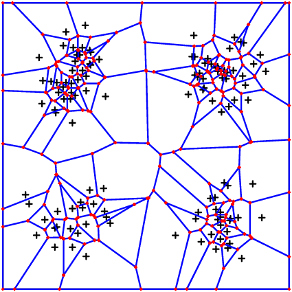
The following two pictures show first a distribution density = x->sin(pi*2*x[1])^2*sin(pi*2*x[2])^2 and the second takes the same density squared.

sin^2 distribution of nodes

sin^4 distribution of nodes

Single Nodes

To instatiate a single node (e.g. if you want to add a specific node to an existing list of nodes) use

# make [1.0, 0.0, 0.5] a valid Voronoi node
VoronoiNode([1.0, 0.0, 0.5])

Example

# This is an example to illustrate VoronoiNodes(number_of_nodes::Int;density)

## First some plot routine ############################
using Plots

function plot_2d_surface(nodes, values)
    # The following two lines are necessary in order for the plot to look nicely
    func = StepFunction(nodes,values)
    new_nodes = vcat([VoronoiNode([k/10,j*1.0]) for k in 0:10, j in 0:1], [VoronoiNode([j*1.0,k/10]) for k in 1:9, j in 0:1])
    append!(nodes,new_nodes)
    append!(values,[func(n) for n in new_nodes])
    
    x = [node[1] for node in nodes]
    y = [node[2] for node in nodes]
    
    p = Plots.surface(x, y, values, legend=false)
    xlabel!("X")
    ylabel!("Y")
    zlabel!("Values")
    title!("2D Surface Graph")
    
    display(p)
end
########################################################

## Now for the main part ################################

my_distribution = x->(sin(x[1]*π)*sin(x[2]*π))^4
my_nodes = VoronoiNodes(100,density = my_distribution, domain=cuboid(2,periodic=[]))
# you may compare the output to the following:
# my_nodes = VoronoiNodes(100,density = x->1.0, domain=cuboid(2,periodic=[]))
println("This generated $(length(my_nodes)) nodes.")
my_vals = map(x->sin(x[1]*π)^2*sin(x[2]*π),my_nodes)
plot_2d_surface(my_nodes,my_vals)

DensityRange

HighVoronoi.DensityRange — Type

DensityRange{S}

provides a rectangular grid of points in a S-dimensional space. It is initialized as follows:

DensityRange(mr::AbstractVector{<:Integer},range)

Here, range can be of the following types:

AbstractVector{Tuple{<:Real,<:Real}}: It is assumed that each entry of range is a tuple (a_i,b_i)

so the range is defined in the cuboid (a_1,b_1) imes... imes(a_{dim},b_{dim})

mr is assumed to have the same dimension as range and the interval (a_i,b_i) will be devided into mr[i] intervalls

AbstractVector{<:Real}: if e.g. range=[1.0,1.0] this will be transferred to range=[(0.0,1.0),(0.0,1.0)]

and the first instance of the method is called

Float64: range will be set range*ones(Float64,length(mr)) and the second instance is called
Tuple{<:Real,<:Real}: range will be set to an array of identical tuple entries and the first version is called

Alternatively, one may call the following method:

DensityRange(mr::Int,range,dimension=length(range))

it is assumed that range is an array or tuple of correct length and mr is replaced by mr*ones(Int64,dimension). If range is not an array, then dimension has to be provided the correct value.

Geometry

The creation and storage of Voronoi geometry data is handled by the following class.

HighVoronoi.VoronoiGeometry — Type

VoronoiGeometry{T}

This is the fundamental struct to store information about the generated Voronoi grid. The geometric data can be accessed using the type VoronoiData. However, there is always the possibility to access the data also via the following fields:

Integrator.Integral: stores the integrated values in terms of a Voronoi_Integral
basic_mesh: stores the fundamental data of nodes and verteces. also stored in Integrator.Integral.MESH
nodes: direct reference to the nodes. Also provided in basic_mesh.nodes

Avoid direct access to the data

Accessing the data directly, that is without calling VoronoiData, is likely to cause confusion or to provide "wrong" information. The reason is that particularly for periodic boundary conditions, the mesh is enriched by a periodization of the boundary nodes. These nodes are lateron dropped by the VoronoiData-Algorithm.

To create a Voronoi mesh it is most convenient to call either of the following methods

HighVoronoi.VoronoiGeometry — Method

VoronoiGeometry(xs::Points,b::Boundary)

This creates a Voronoi mesh from the points xs given e.g. as an array of SVector and a boundary b that might be constructed using the commands in the Boundaries section.

You have the following optional commands:

silence: Suppresses output to the command line when true. The latter will speed up the algorithm by a few percent. default is false.
integrator: can be either one of the following values:
- VI_GEOMETRY: Only the basic properties of the mesh are provided: the verteces implying a List of neighbors of each node
- VI_MONTECARLO: Volumes, interface areas and integrals are calculated using a montecarlo algorithm. This particular integrator comes up with the following additional paramters:
  - mc_accurate=(int1,int2,int3): Montecarlo integration takes place in int1 directions, over int2 volumetric samples (vor volume integrals only). It reuses the same set of directions int3-times to save memory allocation time. Standard setting is: (1000,100,20).
- VI_POLYGON: We use the polygon structure of the mesh to calculate the exact values of interface area and volume. The integral over functions is calculated using the values at the center, the verteces and linear interpolation between.
- VI_HEURISTIC: When this integrator is chosen, you need to provide a fully computed Geometry including volumes and interface areas. VI_HEURISTIC will then use this information to derive the integral values.
- VI_HEURISTIC_MC: This combines directly VI_MONTECARLO calculations of volumes and interfaces and calculates integral values of functions based on those volumes and areas. In particular, it also relies on mc_accurate!
integrand: This is a function f(x) depending on one spatial variable x returning a Vector{Float64}. The integrated values will be provided for each cell and for each pair of neighbors, i.e. for each interface
periodic_grid: This will initiate a special internal routine to fastly create a periodic grid. Look up the section in the documentation.

With density distribution:

VoronoiGeometry(number::Int,b=Boundary();density, kwargs...)

this call genertates a distribution of approsximately number nodes and generates a VoronoiGeometry. It takes as parameters all of the above mentioned keywords (though periodic_grid makes no sense) and all keywords valid for a call of VoronoiNodes(number;domain=b,density=density, ....)

In future versions, there will be an implementation of the parameter cubic=true, where the grid will be generated based on a distribution of "cubic" cells. In the current version there will be a warning that this is not yet implemented.

Advanced methods

VoronoiGeometry(file::String)
VoronoiGeometry(VG::VoronoiGeometry)

Loads a Voronoi mesh from the file or copies it from the original data VG. If integrator is not provided, it will use the original integrator stored to the file. In the second case, if integrand is not provided explicitly, it will use integrand = VG.integrand as standard. Additionally it has the following options:

_myopen=jldopen: the method to use to open the file. See the section on write_jld.
offset: See the section on write_jld.
integrate=false: This will or will not call the integration method after loading/copying the data. Makes sense for using VI_HEURISTIC together with volume=true, area=true and providing values for integrand and integrand. If integrand != nothing but bulk==false or interface==false this parameter will internally be set true.
volume=true: Load volume data from file
area=true: Load interface area data from file
bulk=false: Load integrated function values on the cell volumes from file. When set true and integrand=f is provided the method will compare the dimension of f and of the stored data.
interface=false: Load integrated function values on the interfaces. When set true and integrand=f is provided the method will compare the dimension of f and of the stored data.

Integrators (overview)

As discussed above there is a variety of integrators available to the user, plus some internal integrators that we will not discuss in this manual. The important integrators for the user are:

VI_GEOMETRY: Only the basic properties of the mesh are provided: the verteces and an implicit list of neighbors of each node. This is the fastes way to generate a VoronoiGeometry
VI_MONTECARLO: Volumes, interface areas and integrals are calculated using a montecarlo algorithm introduced by A. Sikorski in VoronoiGraph.jl and discussed in a forthcoming article by Heida, Sikorski, Weber. This particular integrator comes up with the following additional paramters:
- mc_accurate=(int1,int2,int3): Montecarlo integration takes place in int1 directions, over int2 volumetric samples (vor volume integrals only). It reuses the same set of directions int3-times to save memory allocation time. Standard setting is: (1000,100,20).
VI_POLYGON: We use the polygon structure of the mesh to calculate the exact values of interface area and volume. The integral over functions is calculated using the values at the center, the verteces and linear interpolation between. Also this method is to be discussed in the anounced article by Heida, Sikorski, Weber.
VI_HEURISTIC: When this integrator is chosen, you need to provide a fully computed Geometry including volumes and interface areas. VI_HEURISTIC will then use this information to derive the integral values.
VI_HEURISTIC_MC: This combines directly VI_MONTECARLO calculations of volumes and interfaces and calculates integral values of functions based on those volumes and areas. In particular, it also relies on mc_accurate!

It is important to have in mind that the polygon-integrator will be faster in low dimensions, whereas the Montecarlo integrator will outperform from 5 dimensions and higher. However, when volumes and integrals are to be calculated in high dimensions, the VI_HEURISTIC_MC is highly recommended, as it works with much less function evaluations than the VI_MONTECARLO.

Storage

HighVoronoi.write_jld — Method

The data can be stored using the write_jld method:

write_jld(Geo::VoronoiGeometry,filename,offset="";_myopen=jldopen)
write_jld(Geo::VoronoiGeometry,file,offset="")

stores the complete information of a VoronoiGeometry object to a file. This information can later be retrieved using the VoronoiGeometry(file::String, args...) function.

Geo: The Voronoi geometry object to be stored
filename: name of file to store in
file: A file given in a format supporting write(file,"tagname",content) and read(file,"tagname",content)
offset: If several Geometry objects are to be stored in the same file, this will be the possibility to identify each one by a unique name. In particular, this is the key to store several objects in one single file.
_myopen: a method that allows the syntax _myopen(filename,"w") do myfile ....... end. By default the method uses the JLD2 library as this (at the point of publishing this package) has the least problems with converting internal data structure to an output format.

Filname extension

If you want to use the default method, then the filename should end on .jld. Otherwise there might be confusion by the abstract built in julia loading algorithm.

HighVoronoi.load_Voronoi_info — Method

If you want to make sure that the data you load will be rich enough, compact information can be retrieved as follows:

load_Voronoi_info(filname,offset="")

This will print out compact information of the data stored in file filename and the offset offset. Yields dimension, number of nodes, number of internal nodes and the dimension of the stored integrated data. Note that the latter information is of particular importance since here is the highest risk for the user to mess up stored data with the algorithm.

Extraction of `VoronoiData` data for further processing

HighVoronoi.VoronoiData — Type

Using the call

data=VoronoiData(VG)

some data of the Voronoi geometry VG is extracted. Once applied, the data set contains at least the following informations:

nodes::Vector{T}: The original nodes
neighbors::Vector{Vector{Int64}}: For each node nodes[i] the field neighbors[i] contains a sorted list of indeces of all neighboring cells. Multiple appearence of the same node is possible on a periodic grid.

Fields in VoronoiData

Conditionally on what the VoronoiGeometry VG was told to calculate, the set data contains the following additional information:

volume::Vector{Float64}: the volume for each node
area::Vector{Vector{Float64}}: stores for each neighbor neighbors[i][k] of node i in area[i][k] the area of the interface.
bulk_integral::Vector{Vector{Float64}}: the integral over the bulk function
interface_integral::Vector{Vector{Vector{Float64}}}: same as for area but with the integral values of the interface function. In paricular interface_integral[i][k] is of type Vector{Float64}

No request implies empty data field

If the four above data fieds where not requested to be calculated, the vectors have length 0 and any attempt to access their values will eventually result in an error message.

Named Arguments

The call of VoronoiData(VG) provides the following options:

view_only=false: If true this implies that for nodes,volume,area,bulk_integral and interface_integral only views on the internally stored data will be provided. When set to false, deep copies of the of the internal data will be provided. neighbors will always be explicitly defined within this dataset only (i.e. no view)
reduce_to_periodic=true: This erases all data generated from the periodization. It is highly advised to set this option to true as the user will then only see the periodic mesh as one would expect it.
getorientations=false: This is set automatically to true once reduce_to_periodic==true. Once set true the result contains the field orientations::Vector{Vector{T}}, T being the type of d-dimensional vectors originally provided by the nodes of the grid.
getvertices=false: Set to true the field verteces::Vector{Dict{Vector{Int64},T}} will for each node i contain a dictionary [nodes]=>coordinate. furthermore, the field boundary_verteces::Dict{Vector{Int64},boundary_vertex{T}} will contain a list of edges that go to infinity
getboundarynodes=false: Set to true the field boundary_nodes::Dict{Int64,Dict{Int64,T}} will contain a dictionary node=>Dict(boundary=>point), where boundary is the index boundary = length(nodes) + number_of_boundary_plane. When onboundary==false then point will be mirrored version of nodes[node] at the boundary plane number_of_boundary_plane. Otherwise, point is the center of nodes[node] and its mirrored version
onboundary=false: Explained in the last topic. Furthermore, the value is stored in boundary_nodes_on_boundary::Bool
sorted=true: During the reduction of the internal pseude periodic mesh to the fully periodic output, the neighbors (jointly with their respective properties) get sorted by their numbers