Subsections
Applied mathematical finance and stochastic simulation
Collaborator: D. Belomestny,
C. Bender,
A. Kolodko,
D. Kolyukhin,
D. Mercurio,
M. Reiß,
O. Reiß,
K.K. Sabelfeld,
J. Schoenmakers,
V. Spokoiny
Cooperation with: Part (A):
B. Coffey (Merrill Lynch, London, UK),
R. Denk (Universität Konstanz),
R.J. Elliott (University of Calgary, Canada),
H. Föllmer, P. Imkeller, W. Härdle, U. Küchler (Humboldt-Universität
(HU) zu Berlin),
H. Friebel (Finaris, Frankfurt am Main),
H. Haaf, U. Wystup (Commerzbank AG, Frankfurt am Main),
A.W. Heemink, D. Spivakovskaya (Technical University Delft, The
Netherlands),
F. Jamshidian (NIB Capital Den Haag, The Netherlands),
J. Kampen (Ruprecht-Karls-Universität, Heidelberg)
J. Kienitz (Postbank, Bonn),
P. Kloeden (Johann Wolfgang Goethe-Universität Frankfurt am Main),
M. Kohlmann (Universität Konstanz),
C. März, T. Sauder, S. Wernicke (Bankgesellschaft Berlin AG, Berlin),
S. Nair (Chapman & Hall, London, UK),
M. Schweizer (Universität München / ETH Zürich),
S. Schwalm (Reuters FS, Paris, France),
T. Sottinen (University of Helsinki, Finland),
D. Tasche (Deutsche Bundesbank, Frankfurt am Main),
E. Valkeila (Helsinki University of Technology, Finland),
G.N. Milstein (Ural State University, Russia)
Part (B):
P. Kramer (Rensselaer Polytechnic Institute, USA),
O. Kurbanmuradov (Physical Technical Institute, Turkmenian Academy of
Sciences, Ashkhabad, Turkmenistan),
T. Foken (Universit�t Bayreuth),
A. Levykin, I. Shalimova, N. Simonov (Institute of Computational
Mathematics and Mathematical Geophysics, Russian Academy of Sciences,
Novosibirsk, Russia),
M. Mascagni (Florida State University, Tallahassee, USA),
A. Onishuk (Institute of Chemical Kinetics and Combustion, Russian
Academy of Sciences, Novosibirsk, Russia),
O. Smidts (Université Libre de Bruxelles (ULB), Belgium),
H. Vereecken (Forschungszentrum (FZ) J�lich, Institut f�r Chemie und
Dynamik der Geosph�re),
T. Vesala, U. Rannik (Helsinki University, Finland),
W. Wagner (WIAS: Research Group 5)
Supported by:
DFG Research Center MATHEON, project E5;
Reuters Financial Software, Paris;
Bankgesellschaft Berlin AG;
NATO Linkage Grant N978912; DFG
Description:
The central theme of the project Applied mathematical finance
and stochastic simulation
is the quantitative treatment of problems raised by
industry, based on innovative methods and algorithms
developed in accordance with fundamental stochastic principles.
The project concentrates on two main
areas: Applications in financial industry (A)
and the development of basic stochastic models and algorithms
in computational physics (B).
The problems in area (A) include
stochastic modeling of
financial data, valuation of complex
derivative instruments (options),
risk analysis,
whereas in area (B),
stochastic algorithms for boundary value problems of electrostatic and
elasticity potentials,
random velocity field simulation, transport in porous media,
and behavior of complex particle systems like the formation of
charged nanoparticles in a combustion process are studied.
(D. Belomestny, Ch. Bender,
A. Kolodko, J. Schoenmakers).
The valuation of financial derivatives based
on abritrage-free asset pricing involves non-trivial
mathematical problems
in martingale theory, stochastic differential equations, and partial
differential equations.
While its main
principles
are established (Harrison, Pliska, 1981), many numerical problems remain
such as the numerical valuation of (multidimensional)
American equity options
and the valuation of Bermudan-style
derivatives involving the term
structure of interest rates (LIBOR models), [11].
The valuation and optimal exercise of American and Bermudan derivatives
is one of the
most important problems both in theory and practice, see e.g.,
[1].
American options are options contingent on a set of underlyings
which can be exercised at any time in some prespecified future
time interval, whereas Bermudan options may be exercised
at a prespecified discrete set of future exercise dates.
A new development is the valuation of multiple callable products.
In general, the fair price of an American- or Bermudan-style derivative
can be represented as the solution of an optimal stopping problem.
- Iterative methods for Bermudan-style products
In Kolodko and Schoenmakers (2004),
a new iterative procedure for solving the discrete
optimal stopping problem is developed.
The method is based on improving a canonical suboptimal policy
for Bermudan options: Exercise as soon as the cash flow dominates all
underlying Europeans ahead.
An iteration of this policy
produces monotonically increasing
approximations of the Snell envelope from below, which coincide with the
Snell envelope after finitely many steps. The method may be sketched as
follows:
The Bermudan option:
Let
{0, 1,..., k} be the set of Bemudan exercise dates. At one of these dates, say i, the Bermudan option holder may exercise a cash flow Zi.
Construction of the optimal stopping time:
Take a
fixed integer  ,
1
,
1

 k, and an input
stopping family
  =
(
=
( , 0
, 0 i
i k);
k);
 is the stopping (exercise)
time due to policy
  at exercise date i
provided the Bermudan option was not exercised
before date i.
Then consider the intermediate process
Using
 as an exercise
criterion, we define a new family of stopping indexes
 : : |
= |
inf{j : i  j j  k, k,   Zj} Zj} |
|
| |
= |
inf{j : i  j j  k, k,  EjZ EjZ  Zj}, 0 Zj}, 0  i i  k, k, |
|
and consider the process

: =
EiZ
as a next approximation of the Snell envelope. Iterating this procedure
gives then an increasing sequence of stopping families which rapidly
converges to the optimal one.
By duality, the iterative method
induces a convergent sequence
of upper bounds as well.
Contrary to backward
dynamic programming, the presented iterative procedure allows to calculate
approximative solutions with only a few nestings of conditional
expectations and is, therefore, tailor-made for a plain
Monte Carlo implementation. The power of the procedure
is demonstrated for high-dimensional Bermudan products, in particular,
for Bermudan swaptions in a full factor Libor market model.
- Iterative methods for multiple callable products
In a subsequent study, Bender and Schoenmakers (2004), the iterative
procedure of Kolodko and Schoenmakers
is extended for multiple callable options. Moreover,
the stability of the algorithm is proved.
- Modeling American options by consumption processes
An approach for pricing both continuous-time and
discrete-time American options, which is based on the fact that an American
option is equivalent to a European option with a consumption process
involved, is developed in Belomestny and Milstein (2004).
This approach admits the construction of an upper bound (a lower bound) on the
true price using some lower bound (some upper bound).
The method requires the ability of computing the price of a lower bound
at
every position, for instance, by a Monte Carlo procedure. As an example,
let f (t, x) be the
payoff function of an American option, then a lower bound v(t, x) is
given by
v(t, x) = max{f (t, x), ueu(t, x)},
where
ueu(t, x) is the price of the underlying European option which, in
principle, can easily be computed by Monte Carlo.
Then, by the Monte Carlo method, an upper
bound V(t, x) due to this lower bound
is constructed at position (t, x).
A number of effective estimators of the upper and lower bounds with reduced
variance are proposed. The results obtained are supported by numerical
experiments which look promising.
- Pricing Libor Bermudans by Greenian kernel expansions
In a research cooperation with J. Kampen at Heidelberg University we aim
to value Bermudan-style derivatives
in the Libor market model based on higher
order approximation of Greenian kernels. Greenian kernels
are connected with the
(high-dimensional) Libor process and
integration with respect to these kernels will be implemented on sparse grids.
- Option pricing under constraints
The classical theory of option pricing presupposes a frictionless
market. For example, the market is assumed to be liquid, fractions
of shares can be traded, and there are no restrictions on
short selling stocks and borrowing money from the money market
account. To incorporate constraints into a model, one can penalize
violations of the constraints or prohibit violations completely.
In Bender and Kohlmann (2004),
several constructions of penalization processes for
different classes of constraints are presented in the context of a
generalized Black-Scholes market, which yield arbitrage-free,
nonlinear pricing systems. The constraints may be time-dependent,
random, and nonconvex. It is shown that with increasing weight of
the penalization the option prices monotonically tend to the
superhedging price (i.e. the seller's price, when violation of the
constraint is prohibited) due to the monotonic limit theorem for
BSDEs.
- Arbitrage with fractional Brownian motion:
Fractional analogues of the Black-Scholes model have been proposed
in recent years in order to incorporate long memory into market
models. In Bender and Elliot (2004), a binary version of the Wick-fractional
Black-Scholes model is considered and an arbitrage is constructed
in the binary model. It is explained within the binary model why
the no-arbitrage results in continuous time rather stem from
replacing the self-financing condition by an economically doubtful
condition than by the use of the Wick product in the stock price
modeling.
(J. Schoenmakers).
- Book project: Robust Libor modeling and pricing of derivative
products
The research on Libor modeling, robust calibration, and
pricing of exotic products has continued and has led to the monograph of
Schoenmakers (2005). This book contains also much recent work on
Bermudan-style derivatives.
- Interest rate modeling in intrinsic Black-Scholes
economies In the research of Reiß, Schoenmakers, and Schweizer (2004),
the following result is established. If an
economy follows a Black-Scholes dynamics with respect to intrinsic values,
on may define a natural intrinsic asset index, called spherical index,
and with respect to this index there is a testable relationship between
the correlation of index and short rate, and the slope of the yield curve.
This relationship may be used, for example, for
determination of a volatility function in a short rate model.
(D. Belomestny, M. Reiß, V. Spokoiny).
Nowadays, the main focus of financial engineering is the
development and application of probabilistic models that at the
same time capture the main stylized facts of financial time series
and allow robust and fast calibration and pricing methods. Soon
after the introduction of the classical Black & Scholes model for
asset prices, Merton (1976) proposed a more realistic model
incorporating random jumps of the price process. Since then, the
idea of incorporating jumps into the models has become very
popular in mathematical finance, see, e.g., Cont and Tankov (2004),
but the empirical work only concentrated on some very specific
parametric models.
In the work of Reiß and Belomestny (2004), a calibration method
is developed for the classical exponential Lévy model of the
asset price
St =
S0exp(
Lt),
t
0,
L a process with
stationary, independent increments.
From observations of European put and call option prices, the
Lévy-Khinchin characteristic
(b, ,
, ) of the process
L is estimated, which is a nonparametric statistical problem due
to the unknown jump measure
  . In contrast to the
Black-Scholes model, there is in general no unique equivalent
martingale measure in the exponential Lévy model such that a
model fit purely based on historical asset price data is not
meaningful and the main pricing information can only be obtained
from liquid options traded at the market. Cont and Tankov (2004b)
have proposed a penalized nonlinear least squares method to tackle
this calibration problem, which relies on a rather time-consuming
iterative optimization procedure and does not yield provably
optimal convergence results.
Our method is based upon an explicit nonlinear inversion formula
for the price function in the spectral domain and uses the FFT
algorithm. Due to the ill-posedness of the inversion, a spectral
cut-off scheme is employed as regularization method. For an
increasing number of observations the method is provably
rate-optimal, but the rates, even for the parametric drift and
diffusion part, correspond in general to a severely ill-posed
problem. Although this seems discouraging for practical purposes,
simulation studies show that for realistic model
assumptions and observation designs, the calibration works
reasonably well and captures the main features of the underlying
parameters; see picture.
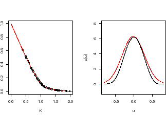
Fig. 1:
Merton model.
Left: Simulated 50 call option prices as a function of strike K
together with the true price curve (red). Right: True and estimated
Lévy densities.
 |
(D. Mercurio, V. Spokoiny).
Since the seminal papers of [66] and [70], modeling the
dynamic features of the variance of financial time series has become one of the
most active fields of research in econometrics. New models, different
applications and extensions have been proposed as it can be seen by consulting,
for example, the monographs [71]. The main
idea behind this strain of research is that the volatility clustering effect
that is displayed by stock or exchange rate returns can be modeled
globally by
a stationary process. This approach is somehow restrictive and it does not fit
some characteristics of the data, in particular the fact that the volatility
process appears to be ``almost integrated'' as it can be seen by usual
estimation results and by the very slow decay of the autocorrelations of
squared returns. Other global parametric approaches have been proposed
by [65] and by [72] in order to include these features
in the model. Furthermore, continuous time models, and in particular diffusions
and jump diffusions, have also been considered; see, for example,
[69] and [64].
However, [79] showed that long memory effects of financial time
series can be artificially generated by structural breaks in the parameters.
This motivates another modeling approach which borrows its philosophy mainly
from the nonparametric statistics. The main idea consists in describing the
volatility clustering effect only by a locally stationary process. Therefore,
only the most recent data are considered and weighting schemes, which can be
themselves either global or local and data driven,
are suggested in order to decrease the dependence of the estimate
on the older observations. Some examples of this approach can be found
in [67],
in [68],
and in [73].
Furthermore,
[76] proposes a new locally
adaptive volatility estimation (LAVE) of the unknown volatility from the
conditionally heteroskedastic returns. The method is based on pointwise
data-driven selection of the interval of homogeneity for every time point. The
numerical results demonstrate a reasonable performance of the new method. In
particular, it slightly outperforms the standard GARCH(1,1) approach.
[74] extend this method to estimating the volatility matrix of
the multiple returns and [78] apply the same idea in the context of
a regression problem.
Mercurio and Spokoiny (2004b) developed another procedure which, however,
applies a similar idea of pointwise adaptive choice of the interval of
homogeneity. The main differences between the LAVE approach and the
new procedure is in the way of testing the homogeneity of the interval
candidate and in the definition of the selected interval. The new
approach is based on the local change-point analysis.
This means that every interval is tested on homogeneity against a change-point
alternative. If the hypothesis is not rejected, a larger interval candidate is
taken. If the change point is detected, then the location of the
change point
is used for defining the adaptive interval while [76]
suggested to take the latest non-rejected interval. The modified procedure allows to improve the
sensitivity of the method to changes of volatility by using the more powerful
likelihood ratio test statistic with the careful choice of the critical level.
In addition, the use of the additional information about the location of the
change point which is delivered by the change-point test, helps to reduce the
estimation bias. Finally, the interpretation of the procedure as a multiple
test against a change-point alternative leads to a very natural method of
tuning the parameters of the procedure.
Another important feature of the proposed procedure is that
it can be easily extended to multiple volatility modeling,
cf. [74].
Suppose that a number of financial time series is observed and the goal is to estimate
the corresponding time-depending volatility matrix. We again assume that the
volatility matrix is nearly constant within some historical time interval
which we identify from the data.
The volatility matrix is estimated in a usual way from the observations which belong
to the detected interval.
The new procedure is shown to be rate-optimal in detecting the volatility
changes and in estimating the smoothly varying volatility function. The
numerical results indicate quite reasonable performance of the procedure.
The assumption of a local constant volatility is very useful in applications to
Value-at-Risk analysis. Indeed, the volatility matrix is assumed nearly constant in
some historical interval and this value of volatility can be extrapolated on
some short time interval of ten working days in the future which is only relevant in the
VaR analysis. Mercurio and Spokoiny (2004) systematically applied this
approach and compared the results with what the standard GARCH (1,1) modeling
delivers, see [75]. It turns out that the local constant method delivers better accuracy
in volatility forecasting leading to a better fit of the prescribed excess rate.
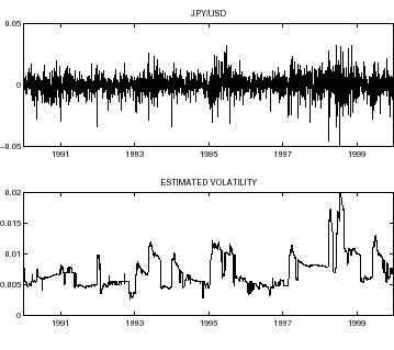
Fig. 2:
Returns and estimated
volatility for the JPY/USD exchange rate
 |
(P. Mathé).
Many financial portfolios are influenced by
a variety of underlyings, but which are only locally correlated. The
valuation of such products leads to high-dimensional integration, but
the integrands possess a small effective dimension.
Prototypically, we exhibit the following situation, describing a
portfolio of a set
{S1, S2,..., Sm}, of m underlyings with
respective shares
 ,
, ,...,
,..., , determining the present value
Vt =

 Sj
Sj.
There are many numerical schemes for the
valuation of such financial products. Often a reasonable approximation
is obtained using the  -
- -normal method for the
forecast of Vt+1 at a future time, knowing Vt, given by
with
 ,
, ,
and
,
and  completely determined by the structure of the portfolio,
and y Gaussian innovations, see [11]. In this case we obtain a
quadratic functional in the underlyings. This remains quadratic when
turning to the independent risk factors. Normally,
  is
sparse.
In cooperation with S. Jaschke, Bundesanstalt
f�r Finanzdienstleistungsaufsicht Bonn, previous analysis of
valuation of the  -
- -normal approximation by means of
stratification, in particular using randomized orthogonal arrays, of large
portfolios was extended to risk analysis. It could be shown that
stratification is a general tool for enhancing known algorithms. This
holds true for randomized orthogonal arrays and also for randomized
digital nets, where recently codes became available for high
dimensions.
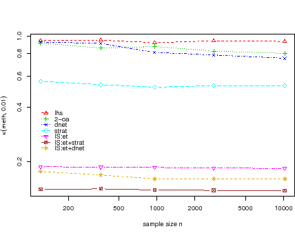
Specifically, the authors introduce a numerical quantity
 (meth, x, n), which
describes the speedup of any chosen method ``meth'', using sample size
n, against plain
Monte Carlo sampling at location x. For specific methods, this
quantity can be shown to be less than 1; thus such methods enhance Monte Carlo simulations.
In Jaschke and Mathé (2004), the theoretical results are combined with an extensive
case study, see Figure 3, based on a portfolio of a German mid-sized
bank.
Fig. 3:
Comparison of the efficiency of different sampling strategies at the
1 % quantile
 |
(J. Schoenmakers).
The method of Milstein, Schoenmakers and Spokoiny [41]
developed in cooperation with the project Statistical
data analysis provides a new transition
density estimator for diffusion processes which is basically root-N
consistent for any dimension of the diffusion process. This estimator,
 (t, x, T, y) = (t, x, T, y) =    K K    t1, y(m)(T), t1, y(m)(T), |
|
|
(1) |
which does not suffer from the ``curse of dimensionality'',
is based on forward simulation of the given process X and reverse
simulation of an adjoint process
(Y, ) which can be constructed
via the (formal) adjoint of the generator of the original process.
The forward-reverse density
estimator in this year was successfully applied to pollution particle
models in the North Sea environment by Spivakovskaya, Heemink,
Milstein and Schoenmakers (2004). In this work,
particle models are used
to simulate the spreading of a pollutant in
coastal waters in case of a calamity at sea.
Many different particle trajectories starting at the point of
release are generated to determine the particle
concentration at some critical
locations after the release.
A standard Monte Carlo method for this essentially
density problem would consume a long CPU
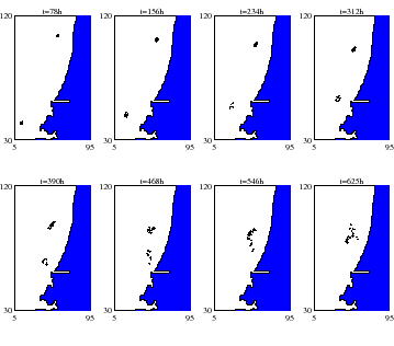
time. However, here it is shown that
the forward-reverse estimator gives superior results, see the figure
below.
Fig. 4:
Forward and reverse pollution particle
simulation near the cost of Holland
 |
In 2004, the research concentrated on the development of new
stochastic models and simulation techniques for solving
high-dimensional boundary value problems with random coefficients
related to the transport in porous media, potential and elasticity
problems, and to the numerical solution of the Smoluchowski equation
governing ensembles of interacting charged particles generated in
a combustion process. New fundamental results were obtained in the
random field simulation: Novel spectral randomization methods and
Fourier/wavelet-based representations for divergenceless random
fields were developed. These models have nice ergodic properties
and can be efficiently implemented in numerical calculations.
The results are presented in the published papers [25],
[28], [55], [63], in the
papers [13], [29], [30] in
press, and in five talks at international conferences.
(K.K. Sabelfeld).
We analyze and compare the efficiency and accuracy of two
simulation methods
for homogeneous random fields with multiscale resolution:
the Fourier-wavelet method and three variants of the
randomization method: (A) without any
stratified sampling of
wavenumber space, (B) stratified sampling of wavenumbers with
equal energy subdivision,
(C) stratified sampling with a logarithmically uniform
subdivision. We focus on fractal Gaussian random fields with
Kolmogorov-type spectra. As known from the previous work
[52], variants (A) and (B) of the randomization method are
only able to generate a self-similar structure function over three
to four decades with reasonable computational effort. By contrast,
variant (C), along with
the Fourier-wavelet method, is able to reproduce accurate
self-similar scaling of the structure function over a number of
decades increasing linearly with computational effort (for our
examples we show that twelve decades can be
reproduced).
We provide some conceptual and numerical comparison
of the various cost contributions to each random field simulation
method (overhead, cost per realization, cost per evaluation).
We expect ergodic properties to be
important in simulating the solutions to partial differential
equations with random field coefficients, and to this end, it is
interesting to
compare the Fourier-wavelet and
various randomization methods in simulating the solution to the
Darcy equation for porous media flow with the heterogeneous
conductivity modeled as a homogeneous random field.
Random functions (generally referred to as random fields)
provide a useful mathematical framework for representing
disordered heterogeneous media in theoretical and computational
studies, [52]. One example is in turbulent transport, where
the velocity field
 (
( ) representing the
turbulent flow is modeled as a random field with statistics
encoding important empirical features, and the temporal dynamics
of the position
 (t) of immersed particles is then
governed by equations involving this random field such as
d (t) (t) |
= |
 (t) dt, (t) dt, |
|
m d (t) (t) |
= |
-    (t) - (t) -  ( ( (t), t) (t), t) dt + dt +  d d (t), (t), |
|
where m is particle mass,  is its friction
coefficient,
kB is Boltzmann's constant, T is the
absolute temperature, and
 (t) is a random Wiener
process representing molecular collisions. Another example is in
transport through porous media, such as groundwater aquifers, in
which the conductivity
K(x) is modeled as random
field reflecting the empirical variability of the porous medium.
The Darcy flow rate
 (
( ) in response to pressure
applied at the boundary is governed by the Darcy equation
 ( ( ) ) |
= |
- K( )grad )grad ( ( ), ), |
|
div |
= |
0, |
|
in which the random conductivity function appears as a
coefficient, and the applied pressure is represented in the
boundary conditions for the internal pressure head  . Our
concern is with the computational simulation of random fields for
applications such as these.
Interesting insights into the dynamics of transport in disordered
media can be achieved already through relatively simple random
models for the velocity field, such as a finite superposition of
Fourier modes, with each amplitude independently evolving
according to an Ornstein-Uhlenbeck process. Here, efficient and
accurate numerical simulations of the flow can be achieved through
application of the well-developed literature on simulating
stochastic ordinary differential equations. We focus instead on
the question of simulating random fields which involve challenging
multiscale structures such as those relevant to porous media and
turbulent flow simulations. Many questions remain open for the
case of Gaussian multiscale random fields, so we confine our
attention to this class.
The paper [30] devoted to this study is to appear in
2005.
(K.K. Sabelfeld, D. Kolyukhin).
In this project, a stochastic
model of a flow in incompressible porous media without the
assumption of smallness of the hydraulic conductivity is
constructed. The hydraulic conductivity is modeled as a
divergenceless random field with a lognormal distribution by a
Monte Carlo method based on the spectral representation of
homogeneous Gaussian random fields described in the previous
section of the present report. The Darcy law and continuity
equation are solved numerically by the successive over-relaxation
method which provides us with detailed statistical characteristics
of the flow. The constructed numerical method is highly efficient
so that we were able to outline the applicability of the spectral
models derived in the first-order approximation.
These results are published partly in [28] and
the results of further study are to be published in [29].
(K.K. Sabefeld).
Stochastic algorithms for solving high-dimensional Dirichlet
problems for the Laplace equation and the system of Lamé
equations are developed. The approach presented is based on the
Poisson integral formula written down for each of a family of
overlapping discs in 2D and spheres in 3D. The original
differential boundary value problem is reformulated in the form of an
equivalent system of integral equations defined on the
intersection surfaces (arcs, in 2D, and caps, in 3D). A random walk
algorithm can be applied then directly to the obtained system of
integral equations where the random walks are living on the
intersecting surfaces (arcs, in 2D, or caps, in 3D). Another
version of a stochastic method is constructed as a discrete random
walk for a system of linear equations approximating our system of
integral equations. We develop two classes of special Monte Carlo
iterative methods for solving these systems of equations which are
a kind of stochastic versions of the Chebyshev iteration method
and SOR method. In the case of classical potential theory, this
approach improves the convergence of the well-known random walk on
spheres method. What is, however, much more important is that this approach
suggests a first construction of a fast convergent finite-variance
Monte Carlo method for the system of Lamé equations.
Consider a homogeneous isotropic medium
G  I Rn with a
boundary
  whose state in the absence of body forces is
governed by the boundary value problem, see, e.g.,
[53]:
  (x) + (x) +  grad div grad div  (x) = 0, x (x) = 0, x  G, G, (y) = (y) =  (y), y (y), y   , ,
|
(2) |
where
 (x) = (u1(x1,..., xn),..., un(x1,..., xn)) is a vector of
displacements, whose components are real-valued regular functions.
The elastic constant
 = (
= ( +
+  )/
)/ is expressed
through the Lamé constants of elasticity
  and
and  .
.
Consider an arbitrary point x with polar coordinates
(r, ) inside a disk K(x0, R). The point y
situated on the circle S(x0, R) has the coordinates
(R,
 ), where
 =
=  +
+  , and z is defined
by z = y - x; note that
  is the angle between the vectors
x and y;
  is the angle between x and z. Define
also the angle
  by
by
 =
=  +
+  .
.
Our method is based on the following solution
representation which we obtained in
[53], [54]:
The solution to Equation (2 ) satisfies
the following mean value relation,
x being an arbitrary point in K(x0, R):
ui(x) =     dSy , i = 1, 2, dSy , i = 1, 2, |
|
|
(3) |
where bij are functions of x, y, explicitly represented as
the entries of the following matrix
B =   . . |
|
|
|
Relation (3 ) reads in the matrix
form:
 (x) = (x) =  p(y;x) B p(y;x) B (y) dS(y) (y) dS(y)
|
(4) |
where
p(y;x) = [R2 - | x - x0|2]/(2 R(| x - y|2) is the kernel of
the Poisson formula for the Laplace equation.
We apply this representation for two overlapping discs,

 being the inner arcs of intersection,
and
 are the corresponding
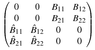
external arcs. We now can derive a system of four
integral equations defined on the arcs
 and
and  . Indeed, let us introduce the notations:
v1(1)(x) = u1(x) and
v1(2)(x) = u2(x) for
x
 , and
v2(1)(x) = u1(x) and
v2(2)(x) = u2(x) for
x
 . Then the system
(4 ) can be written as
 =
= 
 +
+  , or, in more detail,
where the integral operators Bij, i, j = 1, 2, are defined,
according to (3 ), for the points of the first disc
x  K(x0(1)):
Bijv2(j)(
x) =
 p
p(
y;
x)
bij(
x,
y)
v2(j)(
y) d
S(
y),
i,
j = 1, 2 ,
while the integral operators
 , i, j = 1, 2, are defined
for the points of the second disc
x
  K(x0(2)):
 v1(j)
v1(j)(
x) =
 p
p(
y;
x)
bij(
x,
y)
v1(j)(
y) d
S(
y),
i,
j = 1, 2 .
The functions fij are defined analogously:
fi(j)(
x) =

 p
p(
y;
x)
bjk(
x,
y)
gk(
y) d
S(
y),
i,
j = 1, 2 .
We have proved in [55] the following
result:
The integral operator
 of the system (5 ) is a Fredholm operator
with kernels continuous on
x
 and
y
and
y 
 ,
with the same type of singularities at the points of intersection
of the arcs
  and
and  as the singularities in the
case of the Laplace equation. The spectral radius of
  is less
than 1 which ensures the equivalence of system
(5 ) and problem (2 ).
This scheme is extended to the case of n
overlapping spheres. The numerical algorithm based on this
representation is highly efficient. For illustration, we have made
calculations for an elastic polymer consisting of 17 overlapping
discs.
The accuracy of about 0.1 % was achieved in
4.5 min on a personal computer.
(K.K. Sabelfeld).
The use of footprint functions in complex flows has been
questioned because of anomalous behavior reported in recent model
studies. We show that the concentration footprint can be
identified with Green's function of the scalar concentration
equation or the transition probability of a Lagrangian formulation
of the same equation and so is well behaved and bounded by 0 and 1
in both simple and complex flows. The flux footprint in contrast
is not a Green function but a functional of the concentration
footprint and is not guaranteed to be similarly well behaved. We
show that in simple, homogeneous shear flows, the flux footprint,
defined as the vertical eddy flux induced by a unit point source,
is bounded by 0 and 1 but that this is not true in more general
flow fields. An analysis of recent model studies also shows that the
negative flux footprints reported in homogeneous plant canopy
flows are an artefact of reducing a canopy with a complex
source-sink distribution in the vertical to a single layer but
that in canopies on hilly topography the problems are more
fundamental. Finally, we compare footprint inversion with the
direct mass-balance method of measuring surface exchange. We
conclude first that the flux footprint is an appropriate measure
of the area influencing both eddy and advective fluxes on a tower
but that the concentration footprint is the correct measure when
the storage term is important. Second, we deduce that there are
serious obstacles to inverting flux footprints in complex terrain.
The results obtained in [31], [33],
[34] were generalized and published in [63].
The work is done in cooperation with
Prof. Dr. T. Vesala and Dr. U. Rannik (Helsinki University,
Finland), Prof. T. Foken (Universität Bayreuth),
and A. Levykin (Institute of Computational Mathematics
and Mathematical Geophysics, Russian Academy of Sciences, Novosibirsk).
(A. Kolodko, K.K. Sabelfeld).
We deal here with the coagulation of charged
particles, and the concentration is described by the Smoluchowski
equation
 = =    Kijmknimnjk - nlz Kijmknimnjk - nlz  Klizmnim, l > 2; Klizmnim, l > 2;
|
(6) |
nl(r, 0) = nl0(r), nz(z, o) = nz0(z).
The kernel Kijmk is given by
Kijmk =
 Kij
Kij,
where Kij is the usual coagulation coefficient which we
choose as in the case of the free molecular collision regime, and
 is a factor which takes into account the charge on
the particle:

=

in the case of repulsion,

=

in the case of attraction,
where

=

,
kb = 1.38
x 10
-16, is the Boltzmann constant, and
T = 295
K,
and m, k are the values of the charge (integer numbers).
It is seen from the formulation that the dimension of the problem
is enormously increased, compared to the standard Smoluchowski
equation, [26]. Therefore, we suggest a new method
of stochastic simulation, which can be described as follows.
First, we divide the set of all pairs of particles into subclasses
so that in each subclass, the Neumann rejection method can be
effectively applied. The sampling of the subclass is made
according to the direct simulation from a discrete distribution
where the Walker method is applied, see [50].
Some examples of simulations that we have made for the formation of
charged aggregates of nanoparticles by combustion of aluminum
droplets in air are given in [25], and some other
aerosol formation applications are presented by us in
[13].
References:
- F. AITSAHLIA, P. CARR,
American options: A comparison of numerical methods,
in: Numerical Methods in Finance,
L.C.G. Rogers, D. Talay,
Cambridge University Press, 1997, pp. 67-87.
- P. ARTZNER, F. DELBAEN, J.M. EBER, D. HEATH,
Coherent measures of risk,
Math. Finance, 9 (1998), pp. 203-228.
- D. BELOMESTNY, G.N. MILSTEIN,
Monte Carlo evaluation of American options using consumption
processes, working paper, 2003.
- C. BENDER, R.J. ELLIOTT, Arbitrage in a discrete version of the
Wick-fractional Black-Scholes market, Math. Oper. Res., 29
(2004), pp. 935-945.
- C. BENDER, Explicit solutions of a class of linear fractional
BSDEs, to appear in: Systems Control Lett.
,
The restriction of the fractional Itô integral to
adapted integrands is injective, to appear in: Stoch. Dyn.
- C. BENDER, M. KOHLMANN, Superhedging under nonconvex constraints
- A BSDE approach, WIAS Preprint no. 928, 2004.
- C. BENDER, J.G.M. SCHOENMAKERS, An iterative algorithm for
multiple stopping: Convergence and stability, WIAS Preprint no. 991, 2004.
-
R.C. BOSE, A. BUSH,
Orthogonal arrays of strength two and three,
Ann. Math. Statistics, 23 (1952), pp. 508-524.
-
A. BRACE, D. GATAREK, M. MUSIELA,
The market model of interest rate dynamics,
Math. Finance, 7 (1997), pp. 127-155.
- M. BROADIE, J. DETEMPLE,
Recent advances in numerical methods for pricing
derivative securities,
in: Numerical Methods in Finance,
L.C.G. Rogers, D. Talay,
Cambridge University Press, 1997, pp. 43-66.
- CREDIT SUISSE FIRST BOSTON,
CreditRisk+ : A Credit Risk Management Framework,
available at http://www.csfb.com/creditrisk,
1997.
- S. DUBCOV, E. DULCEV, A. LEVYKIN, A. ANKILOV, K.K. SABELFELD, A study of kinetics of aerosol formation in the photolysis of
tungsten hexacarbonyl under low pressure conditions, J. Chemical
Physics, in press.
- P. EMBRECHTS, C. KLÜPPELBERG, T. MIKOSCH,
Modelling Extremal Events, Springer, Berlin, 1997.
- J. FRANKE, W. HÄRDLE, G. STAHL,
Measuring Risk in Complex Stochastic Systems,
Lecture Notes in Statist., 147 (2000), Springer, New
York.
-
P. GAPEEV, M. REISS, A note on optimal
stopping in models with delay, Discussion Paper of
Sonderforschungsbereich 373 no. 47, Humboldt-Universität zu Berlin, 2003.
-
P. GLASSERMAN,
Monte Carlo Methods in Financial Engineering,
Springer, New York, 2003.
-
E. GOBET, M. HOFFMANN, M. REISS,
Nonparametric estimation of scalar diffusions based on low
frequency data, 2003, to appear in: Ann. Statist.
- H. HAAF, O. REISS, J.G.M. SCHOENMAKERS, Numerically
stable computation of CreditRisk+, WIAS Preprint no. 846, 2003,
Journal of Risk, 6 (2004), pp. 1-10.
-
A. HAMEL (ED.), Risikomaße und ihre Anwendungen,
to appear as Report of Martin-Luther-Universität
Halle-Wittenberg.
- M.B. HAUGH, L. KOGAN,
Pricing American options: A duality approach,
working paper, 2001, to appear in: Oper. Res.
- W. HÄRDLE, H. HERWARTZ, V. SPOKOINY,
Time inhomogeneous multiple volatility modelling,
Discussion Papers of Sonderforschungsbereich 373
no. 7, Humboldt-Universität zu Berlin, 2001.
- F. JAMSHIDIAN,
LIBOR and swap market models and measures,
Finance Stoch., 1 (1997), pp. 293-330.
-
S. JASCHKE, P. MATHÉ, Stratified sampling
for risk management, 2004, submitted.
- V.V. KARASEV, A.A. ONISCHUK, O.G. GLOTOV, A.M. BAKLANOV,
A.G. MARYASOV, V.E. ZARKO, V.N. PANFILOV, A.I. LEVYKIN,
K.K. SABELFELD, Formation of charged Al2O3 nanoparticles by
combustion of aluminum in air, Combustion and Flame, 138
(2004), pp. 40-54.
-
A. KOLODKO, K.K. SABELFELD,
Stochastic particle methods for Smoluchowski equation:
Variance reduction and error estimations, Monte Carlo Methods Appl.,
9 (2003), pp. 315-339.
- A. KOLODKO, J.G.M. SCHOENMAKERS,
An efficient dual Monte Carlo upper bound for Bermudan-style
derivatives, WIAS Preprint no. 877, 2003.
-
D. KOLYUKHIN, K.K. SABELFELD, Stochastic Eulerian model for
the flow simulation in porous media. Unconfined aquifers, Monte
Carlo Methods Appl., 10 (2004), pp. 345-357.
-
, Direct numerical solution of
the Darcy equation with random hydraulic conductivity. Mathematics
and computers in simulation, to appear in: Monte Carlo Methods Appl.
-
P. KRAMER, O. KURBANMURADOV, K.K. SABELFELD, Extensions of
multiscale Gaussian random field simulation algorithms, to appear
in: J. Comput. Phys.
-
O. KURBANMURADOV, A. LEVYKIN, U. RANNIK, K.K. SABELFELD,
T. VESALA, Stochastic Lagrangian footprint calculations over a
surface with an abrupt change of roughness height, Monte Carlo
Methods Appl., 9 (2003), pp. 167-188.
- O. KURBANMURADOV, K.K. SABELFELD, O. SMIDTS, H. VEREECKEN, A
Lagrangian stochastic model for transport in statistically
homogeneous porous media, Monte Carlo Methods Appl., 9
(2003), pp. 341-366.
- O. KURBANMURADOV, K.K. SABELFELD, Lagrangian stochastic models
for turbulent dispersion in the atmospheric boundary layer,
Boundary-Layer Meteorology, 97 (2000), pp. 191-218.
- O. KURBANMURADOV, U. RANNIK, K.K. SABELFELD, T. VESALA, Estimation of mean concentration and fluxes by Lagrangian stochastic
models, Math. Comput. Simulation, 54 (2001), pp. 459-476.
-
O. KURBANMURADOV, K.K. SABELFELD, J.G.M. SCHOENMAKERS,
Lognormal approximations to LIBOR market models,
J. Computational Finance, 6 (2002), pp. 69-100.
- P. MATHÉ, Using orthogonal arrays to valuate
 -
-  -normal, working paper, 2003.
- D. MERCURIO, V. SPOKOINY, Estimation of time dependent
volatility via local change-point analysis, WIAS Preprint no. 904, 2004.
-
G.N. MILSTEIN, O. REISS, J.G.M. SCHOENMAKERS,
A new Monte Carlo method for American options,
earlier version: WIAS Preprint no. 850, 2003,
to appear in: Int. J. Theor. Appl. Finance.
-
G.N. MILSTEIN, J.G.M. SCHOENMAKERS,
Monte Carlo construction of hedging strategies against
multi-asset European claims,
Stoch. Stoch. Rep., 73 (2002), pp. 125-157.
- G.N. MILSTEIN, J.G.M. SCHOENMAKERS, V. SPOKOINY,
Forward-reverse representations for Markov chains,
working paper, 2003.
,
Transition density estimation for stochastic differential
equations via forward-reverse representations, Bernoulli, 10
(2004), pp. 281-312.
- G.N. MILSTEIN, M.V. TRETYAKOV,
Numerical analysis of Monte Carlo finite difference evaluation of
Greeks, WIAS Preprint no. 808, 2003.
,
Simulation of a space-time bounded diffusion,
Ann. Appl. Probab., 9 (1999), pp. 732-779.
- K.R. MILTERSEN, K. SANDMANN, D. SONDERMANN,
Closed-form solutions for term structure derivatives with
lognormal interest rates,
J. Finance, 52 (1997), pp. 409-430.
- R.B. NELSON,
An Introduction to Copulas,
Springer, New York, 1999.
-
M. REISS, Nonparametric volatility
estimation on the real line from low-frequency observations, 2003,
submitted.
- O. REISS, Dependent sectors and an extension to
incorporate market risk, in: CreditRisk+ in the Banking Industry,
M. Gundlach, F. Lehrbass, Springer, Berlin/Heidelberg, 2004.
,
Fourier inversion techniques for CreditRisk+, in:
CreditRisk+ in the Banking Industry, M. Gundlach, F. Lehrbass,
Springer, Berlin/Heidelberg, 2004.
- O. REISS, J.G.M. SCHOENMAKERS, M. SCHWEIZER,
From structural assumptions to a link between assets and
interset rates, Preprint no. 136 of DFG Research Center
MATHEON, Technische Universität Berlin, 2004.
- B. RIPLEY, Stochastic Simulation, John Wiley & Sons, New
York, 1987.
- L.C.G. ROGERS,
Monte Carlo valuation of American options,
Math. Finance, 12 (2002), pp. 271-286.
- K.K. SABELFELD, Monte Carlo Methods in Boundary Value
Problems, Springer, Heidelberg, New York, Berlin, 1991.
- K.K. SABELFELD, I. SHALIMOVA, Spherical Means for PDEs,
VSP, Utrecht, The Netherlands, 1997.
,
Random walk methods for static elasticity problems,
Monte Carlo Methods Appl., 8 (2002), pp. 171-200.
- K.K. SABELFELD, I. SHALIMOVA, A. LEVYKIN,
Discrete random walk on large spherical grids generated by
spherical means for PDEs, Monte Carlo Methods Appl., 10
(2004), pp. 559-574.
- J.G.M. SCHOENMAKERS,
Calibration of LIBOR models to caps and swaptions: A way
around intrinsic instabilities via parsimonious structures and a
collateral market criterion, WIAS Preprint no. 740, 2002.
,
Robust Libor Modelling and Pricing of Derivatives Products,
to appear in: Chapman & Hall Fin. Math. Series.
- J.G.M. SCHOENMAKERS, B. COFFEY,
LIBOR rate models, related derivatives and model calibration,
WIAS Preprint no. 480, 1999.
-
,
Stable implied calibration of a multi-factor LIBOR model via a
semi-parametric correlation structure,
WIAS Preprint no. 611, 2000.
-
,
Systematic generation of parametric correlation structures
for the LIBOR market model, Int. J. Theor. Appl. Finance,
6 (2003), pp. 507-519.
- D. SPIVAKOVSKAYA, A.W. HEEMINK, G.N. MILSTEIN, J.G.M. SCHOENMAKERS,
Simulation of particle concentrations in coastal waters using forward and
reverse time diffusion, tentatively accepted for: Advances in
Water Resources.
- D. TASCHE,
Capital allocation with CreditRisk+, in: CreditRisk+
in the Banking Industry, F. Lehrbass, M. Gundlach, Springer, 2004.
- T. VESALA, U. RANNIK, M. LECLERC, T. FOKEN, K.K. SABELFELD, Flux
and concentration footprints, Agricultural and Forest Meteorology,
127 (2004), pp. 111-116.
- T.G. ANDERSEN, L. BENZONI, J. LUND, An empirical
investigation of continuous-time equity return models, J. Finance,
3 (2002), pp. 1239-1284.
- R. BAILLIE, T. BOLLERSLEV, H. MIKKELSEN, Fractionally integrated
generalized autoregressive conditional heteroskedasticity,
J. Econometrics, 74 (1996), pp. 3-30.
- T. BOLLERSLEV, Generalised autoregressive conditional
heteroskedasticity, J. Econometrics, 31 (1986), pp. 307-327.
- M.Y. CHENG, J. FAN, V. SPOKOINY, Dynamic nonparametric
filtering with application to volatility estimation, in: Recent
Advances and Trends in Nonparametric Statistics, M.G. Acritas,
D.N. Politis, eds., Elsevier, Amsterdam, Oxford, Heidelberg, 2003,
pp. 315-333.
- R. DAHLHAUS, S.S. RAO, Statistical inference of
time-varying ARCH processes, Preprint no. 31 of DFG
Schwerpunktprogramm 1214, Universität Bremen, 2003.
- D. DUFFIE, J. PAN, K. SINGLETON, Transform analysis and
asset pricing for affine jump diffusions, Econometrica, 68
(2000), pp. 1343-1376.
- R. ENGLE, Autoregressive conditional heteroskedasticity
with estimates of the variance of U.K. inflation, Econometrica,
50 (1982), pp. 987-1008.
- R. ENGLE, ed., ARCH, Selected Readings, Oxford University
Press, 1995.
- R. ENGLE, T. BOLLERSLEV, Modelling the persistence of
conditional variances, Econometric Rev., 5 (1986),
pp. 1-50, pp. 81-87.
- J. FAN, J. GU, Semiparametric estimation of Value at Risk,
Econom. J., 6 (2003), pp. 260-289.
- W. HÄRDLE, H. HERWARTZ, V. SPOKOINY, Time inhomogeneous
multiple volatility modelling, J. Financial Econom., 1
(2003), pp. 55-95.
- A.J. MCNEIL, R. FREY, Estimation of tail-related risk
measures for heteroskedastic financial time series: An extreme value
approach, J. Empirical Finance, 7 (2000), pp. 271-300.
- D. MERCURIO, V. SPOKOINY, Statistical inference for
time-inhomogeneous volatility models, Ann. Statist., 32 (2004), pp. 577-602.
,
Estimation of time dependent volatility via local change-point
analysis with applications to Value-at-Risk, WIAS Preprint no. 904, 2004.
- D. MERCURIO, C. TORRICELLI, Estimation and arbitrage
opportunities for exchange rate baskets, Applied Econometrics, 35 (2003), pp. 1689-1698.
- T. MIKOSCH, C. STARICA, Is it really long memory we see in
financial returns?, in: Extremes and Integrated Risk
Management, P. Embrechts, ed., Risk Books, UBS Warburg, 2000.
LaTeX typesetting by H. Pletat
2005-07-29
![]() ,
1
,
1![]()
![]()
![]() k, and an input
stopping family
k, and an input
stopping family ![]() =
(
=
(![]() , 0
, 0![]() i
i![]() k);
k);
![]() is the stopping (exercise)
time due to policy
is the stopping (exercise)
time due to policy ![]() at exercise date i
provided the Bermudan option was not exercised
before date i.
Then consider the intermediate process
at exercise date i
provided the Bermudan option was not exercised
before date i.
Then consider the intermediate process
 EiZ
EiZ![]() as an exercise
criterion, we define a new family of stopping indexes
as an exercise
criterion, we define a new family of stopping indexes
 EjZ
EjZ


 dSy , i = 1, 2,
 .
. =
= 
 +
+ 
 =
=  Kijmknimnjk - nlz
 in the case of repulsion,
 in the case of attraction,
 , kb = 1.38 x 10⁻¹⁶, is the Boltzmann constant, and T = 295 K,