TetGen, Version 1.5, User’s ManualAlso available as WIAS Technical Report No. 13, 2013 |
Abstract: TetGen is a software for tetrahedral mesh generation. Its goal is to generate good quality tetrahedral meshes suitable for numerical methods and scientific computing. It can be used as either a standalone program or a library component integrated in other software.The purpose of this document is to give a brief explanation of the kind of tetrahedralizations and meshing problems handled by TetGen and to give a fairly detailed documentation about the usage of the program. Readers will learn how to create tetrahedral meshes using input files from the command line. Furthermore, the programming interface for calling TetGen from other programs is explained.
keywords: tetrahedral mesh generation, Delaunay tetrahedralization, weighted Delaunay triangulation, constrained Delaunay tetrahedralization, mesh quality, mesh refinement, mesh adaption, mesh coarsening
AMS Classification: 65M50, 65N50
TetGen is a robust, fast, and easy-to-use software for generating tetrahedral meshes suitable in many applications.
For a set of 3d (weighted) points, TetGen generates the Delaunay and weighted Delaunay tetrahedralization as well as their duals, the Voronoi diagram and power diagram. For a 3d polyhedral domain, TetGen generates the constrained Delaunay tetrahedralization and an isotropic adaptive tetrahedral mesh of it. Domain boundaries (edges and faces) are respected and can be preserved in the resulting mesh. The shapes of resulting tetrahedra can be provably good for a large class of inputs. One of its main applications is to simulate physical phenomena by numerical methods, such as finite element and finite volume methods. A good quality mesh is essential to achieve high accuracy and efficiency of the simulations.
The algorithms of TetGen are Delaunay-based. They can preserve arbitrary complex geometry and topology. TetGen uses a constrained Delaunay refinement algorithm which guarantees termination and good mesh quality. The robustness of TetGen is enhanced by using advanced technologies developed in computational geometry. A technical paper describing the algorithms and technologies used in TetGen is available [24].
TetGen is an outcome of a long-term research project supported by Weierstrass Institute for Applied Analysis and Stochastics (WIAS). It is continuously developed and improved.
TetGen is written in C++. It uses only C standard library. It is easy to compile and runs on all major 32-bit and 64-bit computer systems. The source code of TetGen is freely available at http://www.tetgen.org. It is distributed under the the terms of the GNU Affero General Public License (AGPL) (v 3.0 or later) or a commercial license provided by WIAS.
The remainder of this section is to give a brief description of the triangulation and meshing problems considered in TetGen, and an overview of the implemented algorithms. For basic usage of TetGen, most of the information are not necessary to know, but Sections 1.2.1 and 1.2.5 contain some necessary guidelines to create correct inputs and to generate quality tetrahedral meshes.
Triangulations are basic geometric structures. A triangulation of a set V of points is a simplicial complex S whose vertex set is a subset of or equal to V, and the underlying space of S is the convex hull of V. Given a point set, there are many triangulations of it. Among them, the Delaunay triangulation is of the most interested one. Its dual is the Voronoi diagram of the point set. Delaunay triangulations and Voronoi diagrams have many nice mathematical properties [1, 12, 7]. They are extensively used in many applications.
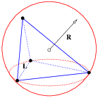
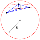
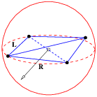
Let V be a set of points in ℝd, σ be a k-simplex (0 ≤ k ≤ d) whose vertices are in V. A circumsphere of σ is a sphere that passes through all vertices of σ. If k = d, σ has a unique circumsphere, otherwise, there are infinitely many circumspheres of σ. We say that σ is Delaunay if there exists a circumsphere of σ such that no vertex of V lies inside it.
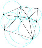
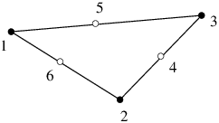
A Delaunay triangulation D of V is a simplicial complex such that all simplices are Delaunay, and the underlying space of D is the convex hull of V [6]. Figure 1 left illustrates a 2d Delaunay triangulation. A 3d Delaunay triangulation is also called a Delaunay tetrahedralization.
A Delaunay triangulation of V is unique if V is in general position, i.e., no d+2 points in V lie on a common sphere. Otherwise, we say that V contains degeneracies, i.e., there are d+2 points in V lie on a common sphere. Degeneracies can be removed by applying an arbitrary small perturbation onto the coordinates of points in V.
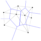
The dual of the Delaunay triangulation is the Voronoi diagram defined on the same vertex set (see Figure 1 right). For any vertex p ∈ V, the Voronoi cell of p is the set of points with distance to p not greater than to any other vertex of V, i.e. it is the set cell(p) = { x ∈ ℝd ; ||x − p|| ≤ ||x − q||, ∀ q ∈ V }, where || · || stands for the Euclidean distance. The Voronoi diagram of V is a subdivision of ℝd into Voronoi cells (some of which may be unbounded) and their faces [27]. It is a d-dimensional polyhedral complex. If the point set V is in general position, there is a one-to-one correspondence between the k-simplices of the Delaunay triangulation and the (d−k)-polyhedra of the Voronoi diagram, where 0 ≤ k ≤ d. In ℝ3, the vertices of the Voronoi diagram are the circumcenters of the tetrahedra of the Delaunay tetrahedralization.
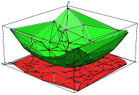
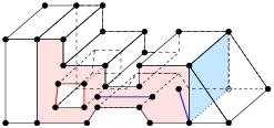
There is a nice relation between a Delaunay triangulation in ℝd and a convex hull in ℝd+1. For any point p = (p0, p1, ⋯, pd−1) ∈ ℝd, define its lifted point p+ = (p0, p1, ⋯, pd−1, pd) ∈ ℝd + 1, where pd = p02 + ⋯ + pd−12. For any point set V ⊂ ℝd, define V+ = {p+ ; p ∈ V} ⊂ ℝd+1 be the lifted point set of V. All points in V+ lie on a paraboloid in ℝd + 1 (see Figure 2 left). The convex hull of V+ is a (d + 1)-dimensional convex polytope P. A lower face of P is a face of P which is on the downside of P (visible by points in V). The Delaunay triangulation of V is the projection of the set of lower faces of P onto d dimensions. Figure 2 right illustrates the relationship when d = 2. A simplex σ is a Delaunay simplex if and only if there exists a hyperplane in ℝd+1 passing through the lifted vertices of σ such that no other lifted vertices in V+ lies below of it. Similarly, the Voronoi diagram of V is the projection of the lower faces of a convex polytope Q ⊂ ℝd+1 such that P and Q are polar to each other [29].
Weighted Delaunay triangulations are generalizations of Delaunay triangulations by replacing the Euclidean distance by “weighted distance”.
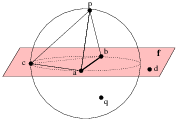
A weighted point, p′ = (p, p2) ∈ ℝd × ℝ, can be interpreted as a sphere centered at p with radius p. The weighted distance between p′ and z′ is
| πp′, z′ = | √ |
| , |
see Figure 3 left for an example. In particular, points in ℝd can be considered weighted points with zero weight.
Two weighted points p′, z′ are orthogonal if their weighted distance is zero, i.e.,
| ||p − z ||2 = (p2 + z2). |
We say that two weighted points are farther than orthogonal when their weighted distance is positive, and closer than orthogonal when the distance becomes an imaginary number.
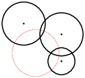
In general, d+1 points in ℝd define a unique circumsphere passing through them. Similarly, d+1 weighted points in ℝd define a unique common orthosphere. When all points have zero weights, their orthosphere is just their circumsphere. Figure 3 (right) gives an example of the orthosphere of three weighted points in two dimensions.
Let V′ ⊂ ℝd × ℝ be a finite set of weighted points. We say a sphere is empty if all weighted points in V′ are farther than orthogonal of it. The weighted Delaunay triangulation of V′ is a simplicial complex D′ such that every simplex has an orthosphere which is empty, and the underlying space of D′ is the convex hull of V′. Obviously, if all the points have the same weight, the weighted Delaunay triangulation is the same as the usual Delaunay triangulation. Note that, a weighted Delaunay triangulation does not necessarily contain all points in V′.
The dual of a weighted Delaunay triangulation is a weighted Voronoi diagram, also called the power diagram [1, 9] of the weighted point set V′. Power diagrams can be similarly defined as the Voronoi diagram by using the weighted distance instead of the Euclidean distance. If no d + 2 weighted points of V′ share a common orthosphere, i.e., it is in general position, then the simplices of the weighted Delaunay triangulation and the cells of the power diagram have a one-to-one correspondence. In ℝ3, the vertices of the power diagram are the orthocenters of the tetrahedra of the weighted Delaunay tetrahedralization.
A weighted Delaunay triangulation of V ⊂ ℝd is also the projection of the set of lower faces of a convex polytope P ⊂ ℝd+1. Any point in p = {p0, ..., pd−1} ∈ V is lifted to a point p′ = {p0, ..., pd−1, pd} ∈ ℝd+1, where pd = p02 + ⋯ + pd−12 − p2 (p is the weight of p). For p ≠ 0, p′ does not lie on a paraboloid in ℝd+1, but is moved vertically downward by p2. A simplex belongs to the weighted Delaunay triangulation of V (i.e., it has an empty orthosphere) if and only if there exits a hyperplane passing through the lifted weighted points of these simplex and no lifted weighted point of V lie below the hyperplane.
Both weighted Delaunay triangulations and power diagrams are called regular subdivisions of point sets [29]. Regular subdivisions have nice combinatorial structures. They are one of the important objects studied in higher-dimensional convex polytopes [29, 5].
Algorithms for generating Delaunay (and weighted Delaunay) tetrahedralizations are well studied in computational geometry [7]. TetGen implemented two algorithms, the Bowyer-Watson algorithm [3, 28] and the incremental flip algorithm [9]. Both algorithms are incremental, i.e., insert points one after another. Both have the worst case runtime O(n2). In most of the practical applications, they are usually very fast. The expected running time of these algorithms is O(n logn) if the points are uniformly distributed in [0,1]3.
The speed of incremental algorithms is very much affected by the cost of point location. TetGen uses a spatial sorting scheme [2] to improve the point location. The idea is to sort the points such that nearby points in space have nearby indices. The points are first randomly sorted in different groups, then points in each group are sorted along the Hilbert curve. Inserting points in this order, each point location can be done in nearly constant time.
TetGen uses Shewchuk’s exact geometric predicates [15] for performing the Orient3D, InSphere, and Orient4D tests. These suffice to guarantee the numerical robustness of generating Delaunay and weighted Delaunay tetrahedralizations. A simplified symbolic perturbation scheme [8] is used to remove the degeneracies.
A tetrahedral mesh is a 3d simplicial complex that is a discrete representation of a 3d continuous space (domain), both in its topology and geometry. Note that a Delaunay tetrahedralization is a tetrahedral mesh of the convex hull of its vertex set. In general, a geometric domain may not be convex and may have arbitrarily complex boundaries.
The input domain of TetGen is modeled by a piecewise linear complex (Section 1.2.1). The focuses of TetGen are the representation of the geometry (the boundary) and the quality of the mesh. TetGen generates several types of tetrahedral meshes to achieve these goals. They are explained in the following subsections.
At first we need a model to represent a 3d domain such that it can be easily described and handled. A 3d piecewise linear complex (PLC) X is a set of cells, that satisfies the following properties:
It is first introduced by Miller, et al. [11], see Figure 4 left for an example.

A 3d PLC non-PLCs
Figure 4: Left: A 3d piecewise linear complex. The left shaded area shows a facet, which is non-convex and has a hole in it. It has also edges and vertices floating in it. The right shaded area shows an interior facet separating two sub-domains. Right: Configurations which are not PLCs.
The boundary of a 3d PLC is the set of cells whose dimensions are less than or equal to 2. A 0-dimensional cell is a vertex. In particular, we call a 1-dimensional cell (an edge) a segment, and a 2-dimensional cell a facet. Each facet of a PLC is a 2d PLC. It may contain holes, segments and vertices in its interior, see Figure 4 left for an example.
PLCs are flexible in describing 3d geometric features. For instance, they permit facets, segments and vertices to float in a domain, or segments and vertices to float in the facet. One purpose of these floating cells is to constrain how the PLC can be meshed, so that boundary conditions may be applied at those cells.
The definition of a PLC disallows illegal intersections of its cells, see Figure 4 right for examples. Two
segments only can intersect at a common vertex that is also in
X. Two facets of X may intersect only at a union of vertices and segments which are also in X.
The underlying space of a PLC X,
denoted | X|, is ∪f ∈ X f,
which is the domain to be triangulated.
A tetrahedral mesh of X,
is a 3d simplicial complex T such that
(1) X and T have the same vertices,
(2) every cell in X is a union of simplices in T, and
(3) | T| = | X|.
Let T be a tetrahedral mesh of a 3d PLC X. The boundary of X is respected by the elements of T, i.e., each segment of X is represented by a union of edges in T, and each facet of X is represented a union of triangles in T.
To distinguish those edges and triangles of T which are on segments and facets of X, we call them boundary edges and boundary faces.
TetGen uses a simple boundary representation (a surface mesh) to represent a 3d PLC. It is explained in Section 5.1.1 and in the file formats .poly and .smesh of TetGen.
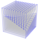
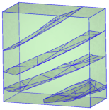
Figure 5 shows two typical surface meshes of 3d PLCs. The following points are useful to know.
A PLC only gives a piecewise linear approximation of a 3d domain. It does not take the curvature of the surfaces into account. When TetGen modifies the surface mesh, it only modifies the linear edges and facets. This is unfortunately a limitation of using PLC.
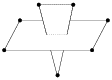
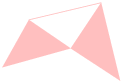
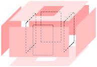
There are 3d polyhedra which may not be tetrahedralized with only its own vertices, two typical examples are shown in Figure 6. Nevertheless, it is always possible to tetrahedralize a polyhedron if Steiner points (which are not vertices of the polyhedron) are allowed.
A Steiner tetrahedralization of a PLC X is a tetrahedralization of X ∪ S, where S is a finite set of Steiner points (disjoint from the vertices of X). TetGen generates Steiner tetrahedralizations of PLCs. Two types of Steiner points are used in TetGen:
In both cases, TetGen tries to generate the Steiner points efficiently and limit the number of Steiner points as small as possible. The optimal locations and the optimal number of Steiner points is still a topic of research.
A fundamental problem in mesh generation is how to enforce a set of constraints, such as edges and triangles, to be preserved or represented by a mesh. These constraints usually describe the special features in the domain boundaries, such as the boundary complex of a PLC, and they are required to be correctly represented in the generated meshes. It is generally referred to the boundary conformity or boundary recovery problem.
Boundary conformity in 2d is very easy. One can enforce any edge (which does not intersect any boundary) into a triangulation. Moreover, it does not need any Steiner point. However, it is very difficult in 3d since it is not always possible to enforce an edge or a triangle into a tetrahedralization without using Steiner points.
TetGen always respects the boundary of the domain. TetGen can generate different types of (Steiner) tetrahedralizations such that input segments and facets of a PLC are respected.
These different types of tetrahedralizations produced by TetGen may find use in different situations. For instances, conforming DTs are desired for applications which need the Delaunay property. While this type of tetrahedralization usually need a large number of Steiner points. CDTs require much less Steiner points. They are an alternative choice of conforming DTs when the applications can accept non-Delaunay elements. Constrained tetrahedralizations are useful in many engineering applications for which the input domain boundaries need to be preserved.
A constrained Delaunay tetrahedralization (CDT) is a variation of a Delaunay tetrahedralization that is constrained to respect the edges and facets of X. CDTs in the plane were introduced by Lee and Lin [10]. Shewchuk [16, 21] generalized them into three or higher dimensions.
In the following, we give two equivalent definitions of constrained Delaunay tetrahedralizations.
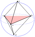
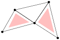
The visibility between two vertices p, q ∈ | X| is called occluded if there is a facet f ∈ X such that p and q lie on opposite sides of the plane that includes f, and the line segment pq intersects this facet (see Figure 7). A tetrahedron t whose vertices are in X is constrained Delaunay if its circumsphere encloses no vertex of X, which is visible from any point in the relative interior of t (see Figure 7 Left).
A tetrahedralization T is a constrained Delaunay tetrahedralization of X if it is a tetrahedralization of X and every tetrahedron of T is constrained Delaunay.
Let s be a triangle in a tetrahedralization T of X. s is said to be locally Delaunay if either it belongs to only one tetrahedron of T, or it is a face of exactly two tetrahedra t1 and t2 and it has a circumsphere which does not enclose any vertex of t1 and t2. Equivalently, the circumsphere of t1 encloses no vertex of t2 and vice versa (see Figure 7 Right). A tetrahedralization T of P is a CDT of P if every triangle in T not included in any facet of P is locally Delaunay.
The definitions of Delaunay tetrahedralization and constrained Delaunay tetrahedralization are almost the same except that, for the CDT, we free the requirement of being locally Delaunay for triangles in the facet. Hence CDTs retain many nice properties of those of Delaunay tetrahedralizations, see [21, 23]. Note that simplices (tetrahedra, triangles, and edges) in a CDT are not always Delaunay.
A CDT of an arbitrary PLC X may not exist [21]. Steiner points are necessary to ensure the existence of a CDT. A Steiner CDT of X is a CDT of X ∪ S, where S ⊂ | X| is a set of Steiner points.
Compared to conforming Delaunay tetrahedralizations, (Steiner) CDTs usually require much less Steiner points.
There is no unique definition of the term “mesh quality". It depends on the intended application and the numerical methods employed, see, e.g. [19].
As a general guideline, elements with very small and large angles (and dihedral angels) should be avoided since they usually downgrade the accuracy and performance of numerical methods.
Figure 8 shows six differently shaped tetrahedra. A tetrahedron shape measure is a continuous function which evaluates the shape of a tetrahedron by a real number. Various tetrahedron shape measures have been suggested, some of them are equivalent.
The most general shape measure for a simplex is the aspect ratio. The aspect ratio, η(τ), of a tetrahedron τ is the ratio between the longest edge length lmax and the shortest height hmin, i.e., η(τ) = lmax/hmin. The aspect ratio measures the “roundness" of a tetrahedron in terms of a value between √2/√3 and +∞. A low aspect ratio implies a better shape. Other possible definitions of aspect ratio exist, such as the ratio between the circumradius and inradius. These definitions are equivalent in the sense that if a tetrahedralization is bounded w.r.t. one of the ratios then it is bounded w.r.t. all the others.
The tetrahedron shape measures used in TetGen are the face angles (angles between two edges) and dihedral angles (angles between two faces) as the shape measures of tetrahedra. They work well with the Delaunay refinement algorithm used in TetGen. Also, the combination of them achieve the same objective as the aspect ratio.
To bound the smallest face angle is equivalent to bound the radius-edge ratio of the tetrahedron. The radius-edge ratio, ρ(τ) of a tetrahedron τ is the ratio between the radius r of its circumscribed ball and the length d of its shortest edge, i.e.,
| ρ(τ) = |
| ≥ |
| , |
where θmin is the smallest face angle of τ, see Figure 9. The radius-edge ratio ρ(τ) is at least √6/4 ≈ 0.612, achieved by the regular tetrahedron. Most of the badly shaped tetrahedra will have a big radius-edge ratio (e.g., > 2.0) except the sliver, which is a type of very flat tetrahedra having no small edges, but nearly zero volume. A sliver can have a minimal value √2/2 ≈ 0.707, hence the radius-edge ratio is not equivalent to aspect ratio (due to the slivers). Nevertheless, the radius-edge ratio is a useful shape measure. It can be shown that if a tetrahedral mesh has a radius-edge ratio bounded for all of its tetrahedra, then the point set of the mesh is well spaced, and each node of the mesh has bounded degree [11, 23].
Each of the six edges of a tetrahedron τ is surrounded by two faces. At a given edge, the dihedral angle between two faces is the angle between the intersection of these faces and a plane perpendicular to the edge. The dihedral angle in τ is between 0∘ and 180∘. The minimum dihedral angle φmin(τ) of τ is a tetrahedron shape measure used by TetGen.
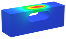
The goal of adaptive mesh generation is to generate a mesh which achieves the desired mesh quality with a small number of mesh elements. In numerical methods, such a mesh gives a good balance between the solution time and the accuracy of the solution, see Figure 10 for an example.
The total number of mesh element is determined by the mesh element sizes, i.e., the diameters of the mesh elements. It is in general no possible to determine a proper mesh element size in advance. It depends on the actual applications and the numerical methods employed.
As a general guideline for adaptive mesh generation, TetGen uses a mesh sizing function. Let X be a 3d PLC. A mesh sizing function H: | X| → ℝ, is a function that maps each point p ∈ | X| to a positive value H(p) which specifies the desired mesh edge lengths at the point location p. Typically, the mesh sizing function can be the geometrical features of the input PLC, an error distribution function obtained from a previous numerical solution, or a user-specified function.
A mesh sizing function H is isotropic if the edge length does not vary with respect to the directions at p, otherwise, it is anisotropic. The current version of TetGen only supports isotropic mesh sizing functions. An ideal sizing function is C∞, ∀ p ∈ | X|. However, in most cases, H is approximated by a discrete function specified at some points in | X|. The size at other points in | X| is obtained by means of interpolation.
TetGen supports several ways of defining a sizing function. It can be defined automatically, explicitly on various sources of volumes, facets, line segments, and points, or through user-defined sizing functions.
All the above ways of defining sizing function can be used at the same time. TetGen will automatically choose the smallest mesh element size. In the last two ways, i.e., defining mesh element sizes on nodes, it is possible to set the size to zero at a node. In this case, the mesh element size at this location is ignored.
Mesh optimization is an essential way for further improving the mesh quality. Typically, it improves one or several objective functions on mesh quality, such as the aspect ratio, minimum or maximum dihedral angles, etc.
Mesh optimization is usually done by applying various local mesh operations which either change the node locations or change the mesh connections. The most frequently used operations are: node smoothing, edge/face swapping, edge contraction, and vertex insertion. These operations are combined according to a schedule to iteratively improve the mesh quality. One can decide to either optimize the whole mesh (global optimization) or only optimize a part of the mesh (local optimization).
TetGen uses mesh optimization after the mesh generation. It locally optimizes the tetrahedral mesh to restore the Delaunay property and to improve the mesh quality. The current version uses the maximum dihedral angle as objective function. It provides options to choose local operations and to restrict the maximum number of iterations in the optimization procedure, see the -O switch.
Algorithms for constructing 3d CDTs were first considered by Shewchuk. In [16], a sufficient condition for the existence of a CDT of a PLC (or a polyhedron) is given. Based on this condition, several algorithms for constructing Steiner CDTs are proposed [18, 20, 26, 25]. TetGen’s CDT algorithm is from Si and Gärtner [26, 25].
The basic algorithm for generating quality tetrahedral meshes is the Delaunay refinement algorithm from Ruppert [13] and Shewchuk [17]. This algorithm generates a quality mesh of Delaunay tetrahedra with no tetrahedra having a radius-edge ratio greater than 2.0 (equivalently, no face angle less than 14.5o). The sizes of tetrahedra are graded from small to large over a short distance. TetGen implemented this algorithm for improving the mesh quality of a CDT of a PLC. In practice, the algorithm generates meshes generally surpassing the theoretical bounds and eliminates tetrahedra with small or large dihedral angles efficiently.
There are two theoretical problems of the basic Delaunay refinement algorithm. First, it does not remove slivers due to the use of radius-edge ratio as the sole tetrahedral shape measure. Second, it may not terminate if the input PLC X contains sharp features, i.e., there are two edges of X meeting at an acute angle, or two facets of X meeting at an acute dihedral angle.
TetGen uses the minimal dihedral angle of tetrahedron as a second shape measure for the Delaunay refinement algorithm, hence slivers are found by this measure and are removed by the above mentioned Delaunay refinement iterations. Since TetGen works with CDTs, it can detect all the sharp features in the CDT in advance. Then it starts the Delaunay refinement process. Tetrahedra at the sharp features are never removed. The modified algorithm in TetGen always terminates. However some badly-shaped tetrahedra near the sharp features may survive.
TetGen accepts a user-defined mesh sizing function to control the mesh element size. If this is given, TetGen will generate an adaptive tetrahedral mesh according to the input mesh sizing function. It uses a constrained Delaunay refinement algorithm [22].
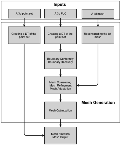
Figure 11 shows a graphic flowchart of the meshing process in TetGen.
Here are the general steps of TetGen to create a (quality) tetrahedral mesh. Many of these steps can be skipped, depending on the command line switches.
This section gives some general information about TetGen. These are not required in order to use TetGen.
TetGen is written entirely in C++, and it only uses the standard C (ANSI) libraries. Hence the code is easily portable and should be compiled by a popular C++ compilers, such as GNU’s gcc/g++, Intel’s and Mircosoft’s C++ compilers. So far, TetGen has been successfully compiled on all major computer architectures and major operating systems (Unix/Linux, Windows, Mac OS) with both 32-bit and 64-bit versions.
The current version of TetGen contains about 25,000 source lines and 7,000 comment lines. These numbers do not include those of Shewchuk’s robust predicates.
TetGen dynamically allocates memory when it is needed. There is no minimum memory requirement to run TetGen. The maximum memory is only limited by the physical memory available from your system. The more memory you have, the larger the mesh you can generate.
For example, the 32-bit version of TetGen used about 694.5 Mega bytes memory to generate the Delaunay tetrahedralization (DT) of a set of 2,000,000 (two million) points randomly distributed inside a unit cube. This DT has 13,504,899 tetrahedra. This is approximately 364 bytes per vertex or 54 bytes per tetrahedron. In other words, with 4 Giga byte memory, a maximum Delaunay tetrahedralization may be generated by the 32-bit version of TetGen having approximately 11,799,360 (ca. 11 million) vertices or 79,536,431 (ca. 79 million) tetrahedra.
More memory is needed in generating quality tetrahedral meshes. The extra memory is used to store boundary information and working arrays of algorithms. For example, the 32-bit version of TetGen used about 770 Mega bytes memory to generate a quality tetrahedral mesh with 2,000,000 (two million) vertices and 12,237,300 tetrahedra.
So far, the largest quality tetrahedral mesh was generated by the 64-bit version of TetGen. It contains 1,007,700,944 (ca. 1 billion) vertices, and 6,454,556,696 (ca. 6.45 billion) tetrahedra. TetGen used about 905.7 Giga bytes memory on generating this mesh, see Table 2.
When generating Delaunay tetrahedraliations, the worst case running time of TetGen is O(n2), where n is the input number of vertices. However, this only happens for some very special point sets. For most point sets appearing in applications, TetGen runs in almost O(n logn) time, see Table 1.
The CPU time required to obtain the quality tetrahedral mesh is obviously related to the complexity of the geometry and topology of the inputs, as well as the command line switches and parameters specified. Nevertheless, the running time of TetGen increases almost linearly with respect to the output number of mesh elements, see Table 2.
This section gives some practical information regarding the performance of TetGen. In particular, Table 1 and Table 2 report the statistics of some test runs of TetGen. The used version of TetGen was a 64-bit version compiled by GNU gcc/g++ version 4.7.2 with the −O3 (optimization) switch. The used computer was a computer of WIAS (erhard-03) with Intel(R) Xeon(R) Ten-Core 2.40GHz CPU, 1,024 Giga byte memory, and SuSE Linux. The given CPU times exclude the file I/O time. Comparisons of TetGen with other programs are available in paper [24].
Table 1 shows the statistics of TetGen on creating Delaunay tetrahedralizations. Three random point sets of different sizes are used in these tests. They are generated by the tool rbox (command: rbox -D3 xxx) in the program qhull (http://www.qhull.org). It is well known that the Delaunay tetrahedralizations of random point sets have linear complexity. Both memory usage and CPU time of TetGen are quasilinear.
Table 2 shows the statistics of TetGen on creating quality tetrahedral meshes. The input of these tests is a 3d unit cube with 8 vertices and 6 facets described in file cube.smesh. The resulting meshes were generated by using the command: tetgen -pqa# -x1000000 cube.smesh, where “-a#” specifies a very small tetrahedron volume constraint, and “ -x1000000” specifies a user-defined memory allocation size.
volume # of points # of tets used memory CPU time constraint (output) (output) (Mega bytes) (seconds) 1.0×10⁻⁷ 3,023,518 18,744,549 2,904 126 1.0×10⁻⁸ 29,412,255 186,090,870 27,599 1,374 1.0×10⁻⁹ 290,323,148 1,854,336,524 268,781 12,124 5.0×10⁻¹⁰ 579,301,396 3,706,331,655 534,386 26,872 2.87×10⁻¹⁰ 1,007,700,944 6,454,556,696 927,449 44,261
Table 2: Statistics of TetGen on generating quality tetrahedral meshes.
When running TetGen, errors may happen. In this case, TetGen may fail to generate a mesh. The typical reasons that cause failures of TetGen may be one of the follows:
In most cases TetGen is able to detect the error. If TetGen is running as a standalone program and if an error is detected, then TetGen will report a message that describes the error possibly together with a suggestion to fix it, and terminate. Below is an example of such a message.
Found two segments intersect each other.
  1st: [13,7] 1.
  2nd: [1114,1113] 1.
A self-intersection was detected. Program stopped.
Hint: use -d option to detect all self-intersections.
If TetGen is running as a library, i.e., it is called inside other program, then the error message will not be seen, and TetGen will throw an error index (integer), which can be catched by the standard C++ exception handler try and catch. A list of error indices and messages are provided in the Appendix.
When TetGen terminates on error, it automatically releases the used memory before terminating itself. This avoids potential memory leak when calling TetGen multiple times.
TetGen is distributed in its source code (written in C++). The latest version of TetGen is available at http://www.tetgen.org.
Section 3.1 briefly explains how to compile TetGen into an executable program or a library.
Once TetGen is compiled, and assume you have the executable file, tetgen (or tetgen.exe in Windows), you can start testing TetGen with the included example file by following the tutorial in Section 3.2.
TetGen does not have a graphic user interface (GUI). The TetView program can be used to visualize the input and output of TetGen. Alternatively, other popular mesh viewers are supported, see Section 3.3.
The downloaded archive should include the following files:
| README | General information. |
| LICENSE | Copyright notices. |
| tetgen.h | C++ header file of TetGen. |
| tetgen.cxx | C++ source file of TetGen. |
| predicates.cxx | C++ source of Shewchuk’s predicates. |
| makefile | make file for compiling TetGen. |
| CMakeLists.txt | cmake file for compiling TetGen. |
| example.poly | An example input file. |
The file predicates.cxx is a modified C++ version of Shewchuk’s robust geometric predicates http://www.cs.cmu.edu/~quake/robust.html.
To compile TetGen, use a C++ compiler for the system on which TetGen will be used, such as GNU’s g++, or Microsoft C++ on MS Windows systems. TetGen may be compiled into an executable program or a library, which can be embedded into another program.
The easiest way to compile TetGen is to edit and use the included makefile. Before compiling, put all source files, tetgen.h, tetgen.cxx, and predicates.cxx and the makefile into one directory (usually they are), read the makefile, which describes your options, and edit it accordingly.
You should at least specify the C++ compiler and the level of optimization. By default, the GNU C++ compiler (g++) is used, and there is no optimization is used.
Once you have done this, type make to compile TetGen into an executable program or type make tetlib to compile TetGen into a library. The executable file tetgen or the library libtet.a appears in the same directory as the makefile.
Alternatively, the files are usually easy to compile directly on the command line. Assume you’re using g++, first compile the file predicates.cxx to get an object file:
g++ -c predicates.cxx
To compile TetGen into an executable file, use the following command:
g++ -o tetgen tetgen.cxx predicates.o -lm
To compile TetGen into a library, the symbol TETLIBRARY is needed:
  g++ -DTETLIBRARY -c tetgen.cxx
  ar r libtet.a tetgen.o predicates.o
Some additional remarks to get an efficient executable version of TetGen.
Here is an example to get an optimized version of TetGen using GNU’s C++ compiler:
  g++ -O3 -DNDEBUG -c predicates.cxx
  g++ -O3 -DNDEBUG -o tetgen tetgen.cxx predicates.o -lm
As an alternative, one can compile TetGen using cmake (www.cmake.org). It simplifies the compilation of TetGen with different compilers and architectures (Linux, MacOSX, and MS Windows) at the same time.
Using the provided file CMakeLists.txt, the simplest sequence of commands is:
  cd <tetgen-directory>
  mkdir build
  cd build
  cmake ..
  make
When the compilation is finished, you should get both of the executable file tetgen and the library libtet.a under the directory build.
To get a debug version of TetGen, use the following commands
  cd <tetgen-directory>
  mkdir build
  cd build
  cmake -DCMAKE_BUILD_TYPE=Debug ..
  make
The default is cmake -DCMAKE_BUILD_TYPE=Release ...
To specify a compiler, do
CXX=icpc cmake -DCMAKE_BUILD_TYPE=Debug ..
TetGen default uses Shewchuk’s robust geometric predicates which perform exact floating-point arithmetic (predicates.cxx). The arithmetic are based on the IEEE 754 floating-point standard. However, some processors may not default use this standard for floating-point representations and arithmetic. If so, a configuration is needed to correctly execute the predicates. It is described on its website http://www.cs.cmu.edu/~quake/robust.pc.html for details.
Below are my own experience in using Shewchuk’s predicates.
Alternatively, TetGen can use other robust predicates developed in computational geometry, such as the filtered robust predicates in CGAL (http://www.cgal.org). TetGen includes the interface to the CGAL’s predicates in the file predicates.cxx. It uses the following kernel,
#include <CGAL/Exact_predicates_inexact_constructions_kernel.h>
In this section, we show how to use CGAL’s predicates in TetGen. The following steps are needed.
cd CGAL-x.y # go to CGAL directory
cmake . # configure CGAL
make # build the CGAL libraries
If you have any problems in compiling CGAL, please see CGAL’s manual about installation. Once CGAL is compiled, make sure that you get the new file compiler_config.h inside the directory CGAL-x.y/include/CGAL.
BOOST=/opt/local/include
GMP_LIB=/opt/local/lib
CGAL_INC=$(HOME)/Programs/CGAL/CGAL-4.1/include
BOOST should point to the directory containing the boost library. Version 1.35 or later is required. GMP_LIB should point to the directory containing the library GMP, - the GNU Multiple Precision Arithmetic Library. And CGAL_INC should point to the C++ headers of CGAL’s library.
g++ -I$(BOOST) -I$(CGAL_INC) -DUSE_CGAL_PREDICATES \
  -O3 -c predicates.cxx
g++ -O3 -o tetgen tetgen.cxx predicates.o -L$(GMP_LIB) -lgmp
TetGen gives a short list of command line options if it is invoked without arguments (that is, just type tetgen). A brief description of the usage is printed by invoking TetGen with the -h switch:
tetgen -h
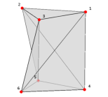
The enclosed example file, example.poly, is a simple 3d mesh domain (a PLC), see Figure 24. Try out TetGen using:
tetgen -p example.poly
With the -p switch, TetGen will read the file, i.e., example.poly, and generate its constrained Delaunay tetrahedralization. The resulting mesh is saved in four files: example.1.node, example.1.ele, example.1.face, and example.1.edge, which are a list of mesh nodes, tetrahedra, boundary faces, and boundary edges, respectively. The file formats of TetGen are described in Section 5. The screen output of the above command looks like this:
Opening example.poly.
Delaunizing vertices...
Delaunay seconds:  0.000864
Creating surface mesh ...
Surface mesh seconds:  0.000307
Constrained Delaunay...
Constrained Delaunay seconds:  0.000325
Removing exterior tetrahedra ...
Exterior tets removal seconds:  8.6e-05
Optimizing mesh...
Optimization seconds:  6.4e-05

Writing example.1.node.
Writing example.1.ele.
Writing example.1.face.
Writing example.1.edge.

Output seconds:  0.000663
Total running seconds:  0.002451

Statistics:

  Input points: 28
  Input facets: 23
  Input segments: 44
  Input holes: 2
  Input regions: 2

  Mesh points: 28
  Mesh tetrahedra: 68
  Mesh faces: 160
  Mesh faces on facets: 50
  Mesh edges on segments: 44
The above mesh is pretty coarse, and contains many badly-shaped (e.g., long and skinny) tetrahedra. Now try:
tetgen -pq example.poly
The -q switch triggers the mesh refinement such that Steiner points are added to remove badly-shaped tetrahedra. The resulting mesh is contained in the same four files as before. However, now it is a quality tetrahedral mesh whose tetrahedra have no small face angle less than about 14o (the default quality value). The screen output of the above command looks like this:
Opening example.poly.
Delaunizing vertices...
Delaunay seconds:  0.000384
Creating surface mesh ...
Surface mesh seconds:  0.000181
Constrained Delaunay...
Constrained Delaunay seconds:  0.000163
Removing exterior tetrahedra ...
Exterior tets removal seconds:  0.000368
Refining mesh...
Refinement seconds:  0.009291
Optimizing mesh...
Optimization seconds:  0.000517

Writing example.1.node.
Writing example.1.ele.
Writing example.1.face.
Writing example.1.edge.

Output seconds:  0.004716
Total running seconds:  0.015802

Statistics:

  Input points: 28
  Input facets: 23
  Input segments: 44
  Input holes: 2
  Input regions: 2

  Mesh points: 216
  Mesh tetrahedra: 689
  Mesh faces: 1587
  Mesh faces on facets: 430
  Mesh edges on segments: 126
  Steiner points inside domain: 1
  Steiner points on facets:  105
  Steiner points on segments:  82
Now try to run:
tetgen -pq1.2V example.poly
TetGen will again generate a quality mesh, which contains more points than the previous one, and all tetrahedra have radius-edge ratio bounded by 1.2, i.e., the element shapes are better than those in the previous mesh. In addition, TetGen prints a mesh quality report (due to the -V switch) which looks as below:
Mesh quality statistics:

  Smallest volume:       0.00059866   |  Largest volume:          0.09363
  Shortest edge:               0.25   |  Longest edge:             1.4142
  Smallest asp.ratio:        1.3255   |  Largest asp.ratio:        10.169
  Smallest facangle:         24.898   |  Largest facangle:       126.8698
  Smallest dihedral:         8.6045   |  Largest dihedral:       163.4980

  Aspect ratio histogram:
         < 1.5       :        23      |      6 - 10         :        26
     1.5 - 2         :       364      |     10 - 15         :         1
       2 - 2.5       :       480      |     15 - 25         :         0
     2.5 - 3         :       248      |     25 - 50         :         0
       3 - 4         :       125      |     50 - 100        :         0
       4 - 6         :        56      |    100 -            :         0
  (A tetrahedron's aspect ratio is its longest edge length divided by its
    smallest side height)

  Face angle histogram:
      0 -  10 degrees:         0      |     90 - 100 degrees:       465
     10 -  20 degrees:         0      |    100 - 110 degrees:       132
     20 -  30 degrees:       188      |    110 - 120 degrees:        54
     30 -  40 degrees:      1059      |    120 - 130 degrees:         5
     40 -  50 degrees:      1704      |    130 - 140 degrees:         0
     50 -  60 degrees:      1865      |    140 - 150 degrees:         0
     60 -  70 degrees:      1609      |    150 - 160 degrees:         0
     70 -  80 degrees:      1105      |    160 - 170 degrees:         0
     80 -  90 degrees:       736      |    170 - 180 degrees:         0

  Dihedral angle histogram:
       0 -  5 degrees:         0      |     80 - 110 degrees:      1831
       5 - 10 degrees:         2      |    110 - 120 degrees:       274
      10 - 20 degrees:       150      |    120 - 130 degrees:       193
      20 - 30 degrees:       266      |    130 - 140 degrees:       105
      30 - 40 degrees:       643      |    140 - 150 degrees:        62
      40 - 50 degrees:      1056      |    150 - 160 degrees:        52
      50 - 60 degrees:      1213      |    160 - 170 degrees:        24
      60 - 70 degrees:      1121      |    170 - 175 degrees:         0
      70 - 80 degrees:       946      |    175 - 180 degrees:         0
Instead of using the -q switch to get a finer mesh, one can use the -a switch to impose a maximum volume constraint on the resulting tetrahedra. By doing so, no tetrahedron in the resulting mesh has volume bigger than the specified value after -a. Try to run the following command.
tetgen -pq1.2Va1 example.poly
Now the resulting mesh should contain much more vertices than the previous one. Besides of -q and -a switches, TetGen provides more switches to control the mesh element size and shape. They are described in Section 4.
To compute the Delaunay tetrahedralization and convex hull of the point set of this PLC, try this:
  cp example.poly example.node
  tetgen example.node
The Delaunay tetrahedralization is saved in example.1.node and example.1.ele. The convex hull is represented by a list of triangles in file example.1.face.
All these meshes and Delaunay tetrahedralizations can be visualized by the programs introduced in the next section.
Detailed descriptions of the command line switches and file formats are found in Section 4 and 5.
TetView is a graphic interface for viewing piecewise linear complexes and simplicial meshes. It can read the input and output files of TetGen and display the objects. It also shows other information as well, such as boundary types and materials. The interactive GUI allows the user to manipulate (i.e., rotate, translate, zoom in/out, cut, shrink, etc.) the viewing objects easily through either mouse or keyboard. TetView can save the current window contents into high quality encapsulated postscript files. Most of the figures of this document were produced by TetView.
TetView is freely available from http://www.tetgen.org/tetview.html. You will find a list of precompiled executable versions on different platforms. Download the one corresponding to your system.
To show the PLC in example.poly, first copy the executable file (tetview) to the directory where you have this file. It is loaded by running:
tetview example.poly
And the following command will display the mesh (in files example.1.node, example.1.ele, and example.1.face):
tetview example.1.ele
The instruction for using TetView can be found on the above website.
TetGen can export its tetrahedral mesh into the .mesh format. It can be then visualized by the software Medit, which is freely available from http://www.ann.jussieu.fr/~frey/logiciels.
For viewing mesh under Medit, add a -g switch in the command line. TetGen will additionally output a file named example.1.mesh, which can be read and rendered directly by TetGen. Try running:
  tetgen -pg example.poly
  medit example.1
Alternatively, TetGen can also output its tetrahedral mesh into the .vtk format by adding the switch -k, i.e.,
tetgen -pk example.poly
It will output a file named example.1.vtk. It can then be visualized by the software Paraview: http://www.paraview.org.
This section describes the use of TetGen as a stand-alone program. It is invoked from the command line with a set of switches and an input file name. Switches are used to control the behavior of TetGen and to specify the output files. In correspondence to the different switches, TetGen will generate the Delaunay tetrahedralization, or the constrained (Delaunay) tetrahedralization, or the quality conforming (Delaunay) mesh, etc.
tetgen [-pYrq_Aa_miO_S_T_XMwcdzfenvgkJBNEFICQVh] input_file
Underscores indicate that numbers may optionally follow certain switches. Do not leave any space between a switch and its numeric parameter. These switches are explained in Section 4.2.
input_file can be different files depending on the switches you use. If no command line switch is used, it must be a file with extension .node which contains a list of 3d points and the Delaunay tetrahedralization of this point set will be generated.
If the -p switch is used, input_file must be a file with one of the following extensions: .poly, .smesh, .off, .stl, .ply, and .mesh, which describes the boundary (a surface mesh) of a 3d piecewise linear complex. The boundary constrained (Delaunay) tetrahedralization of this object will be generated. If the -q switch is used simultaneously, a boundary conforming quality tetrahedral mesh will be generated.
If the -r switch is used, an existing tetrahedral mesh will be read. You must supply .node and .ele files which describe the tetrahedral mesh. Optionally a .face and a .edge file can be supplied which contain the boundary faces and edges of the mesh. input_file can have no file extension.
If the switch -q is applied, the mesh will be refined with respect to the new quality measure and variant constraints. Optionally, and a .vol, a .mtr, and a .var file can be supplied which contain the mesh element size control information.
File formats are described in Section 5.
An overview of all command line switches and a short description follow. These switches are shown by invoking TetGen without any switch and input file. Detailed descriptions of these switches are given in the following subsections.
| -p | Tetrahedralizes a piecewise linear complex (PLC). |
| -Y | Preserves the input surface mesh (does not modify it). |
| -r | Reconstructs a previously generated mesh. |
| -q | Refines mesh (to improve mesh quality). |
| -R | Mesh coarsening (to reduce the mesh elements). |
| -A | Assigns attributes to tetrahedra in different regions. |
| -a | Applies a maximum tetrahedron volume constraint. |
| -m | Applies a mesh sizing function. |
| -i | Inserts a list of additional points. |
| -O | Specifies the level of mesh optimization. |
| -S | Specifies maximum number of added points. |
| -T | Sets a tolerance for coplanar test (default 10−8). |
| -X | Suppresses use of exact arithmetic. |
| -M | No merge of coplanar facets or very close vertices. |
| -w | Generates weighted Delaunay (regular) triangulation. |
| -c | Retains the convex hull of the PLC. |
| -d | Detects self-intersections of facets of the PLC. |
| -z | Numbers all output items starting from zero. |
| -f | Outputs all faces to .face file. |
| -e | Outputs all edges to .edge file. |
| -n | Outputs tetrahedra neighbors to .neigh file. |
| -v | Outputs Voronoi diagram to files. |
| -g | Outputs mesh to .mesh file for viewing by Medit. |
| -k | Outputs mesh to .vtk file for viewing by Paraview. |
| -J | No jettison of unused vertices from output .node file. |
| -B | Suppresses output of boundary information. |
| -N | Suppresses output of .node file. |
| -E | Suppresses output of .ele file. |
| -F | Suppresses output of .face and .edge file. |
| -I | Suppresses mesh iteration numbers. |
| -C | Checks the consistency of the final mesh. |
| -Q | Quiet: No terminal output except errors. |
| -V | Verbose: Detailed information, more terminal output. |
| -h | Help: A brief instruction for using TetGen. |
Given a set of 3d points or weighted points, TetGen generates the Delaunay tetrahedralization or the weighted Delaunay tetrahedralization of the point set. It can also output the Voronoi diagram or the power diagram.
Save the set of points in a .node file, e.g., test.node. Run TetGen using the command:
tetgen test.node
This command generates the Delaunay tetrahedralization (DT) of this point set. Below is a screen output of TetGen:
Opening test.node.
Delaunizing vertices...
Delaunay seconds:  0.001695

Writing test.1.node.
Writing test.1.ele.
Writing test.1.face.

Output seconds:  0.001555
Total running seconds:  0.003615

Statistics:

  Input points: 100

  Mesh points: 100
  Mesh tetrahedra: 514
  Mesh faces: 1057
  Mesh edges: 642
  Convex hull faces: 58
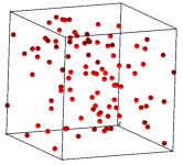
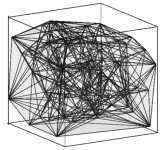
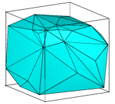
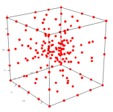
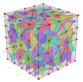
Figure 12 shows an example of an input point set (100 vertices) and the generated DT and its convex hull.
The default outputs of TetGen are three files listed in Table 3.
The set of all faces and edges of the DT can be obtained by adding the output switches -f (output all faces) and -e (output all edges), respectively. For example, by the following command
tetgen -fe test.node
TetGen will output the four files listed in Table 4.
test.1.node The list of vertices (same as input) of the DT. test.1.ele The list of tetrahedra of the DT. test.1.face The list of all faces of the DT. Convex hull faces have a face marker ‘1’. Interior faces have a face marker ‘0’. test.1.edge The list of all edges of the DT. Convex hull edges have an edge marker ‘1’. Interior edges have an edge marker ‘0’.
Table 4: The output files by the command: tetgen -fe test.node.
The adjacency graph of the list of tetrahedra of the DT can be obtained by adding the -n switch in the command line. An additional file, test.1.neigh, will be output by TetGen, see file format .neigh for details.
The -w switch creates a weighted Delaunay tetrahedralization from a set of weighted points. Remember that a weighted point is defined as p′ = {px, py, pz, px2 + py2 + pz2 − w} ∈ ℝ4, where w is the weight (a real value) of the point p = {px, py, pz} ∈ ℝ3 [7].
Save the set of weighted points in a .node file. The points in .node file must have at least one attribute, and the first attribute of each point is its weight. To generate a weighted DT of this point set, run TetGen with the following command:
tetgen -w test.node
The weighted Delaunay tetrahedralization and its convex hull are saved in the files with the same names as is listed in Table 3. Note that some of the points in test.1.node may not belong to any tetrahedron.
The Voronoi diagram or the power diagram of the point set is obtained by taking the dual of the generated Delaunay or weighted Delaunay tetrahedralization, see Figure 13 for an example.
By adding a -v switch in the command line, TetGen outputs the Voronoi diagram or the power diagram in the four files shown in Table 5:
The .v.node file has the file format as a .node file. The file formats of .v.edge, .v.face, and .v.cell are described in the file format section.
Note that the switches -w and -v are only used for a point set.
The -p switch reads a boundary description (a surface mesh) of a 3d piecewise linear complex (PLC) stored in file .poly or .smesh and generates a tetrahedral mesh of the PLC.
By default, TetGen generates a constrained Delaunay tetrahedralization (CDT) of the PLC. Here is an example of creating a CDT of the PLC named cami1a.poly (Figure 14 left). Run the following command:
tetgen -p cami1a.poly
This will produce the CDT of the PLC shown in Figure 14 middle. Below is a screen output of TetGen:
Opening cami1a.poly.
Opening cami1a.node.
Delaunizing vertices...
Delaunay seconds:  0.019862
Creating surface mesh ...
Surface mesh seconds:  0.002374
Constrained Delaunay...
Constrained Delaunay seconds:  0.012435
Removing exterior tetrahedra ...
Exterior tets removal seconds:  0.000783
Optimizing mesh...
Optimization seconds:  0.000662

Writing cami1a.1.node.
Writing cami1a.1.ele.
Writing cami1a.1.face.
Writing cami1a.1.edge.

Output seconds:  0.003398
Total running seconds:  0.039744

Statistics:

  Input points: 460
  Input facets: 884
  Input segments: 690
  Input holes: 0
  Input regions: 0

  Mesh points: 542
  Mesh tetrahedra: 1678
  Mesh faces: 3904
  Mesh faces on facets: 1118
  Mesh edges on segments: 772
  Steiner points on segments:  82
From the mesh statistics of the output (the last line), we can see that TetGen added 82 Steiner points on the segments of the PLC.
If the -Y switch is used simultaneously, the input boundary edges and faces of the PLC are preserved in the generated tetrahedral mesh. Steiner points (if there exists any) appear only in the interior space of the PLC. For example, run the following command:
tetgen -pY cami1a.poly
This will produce a tetrahedral mesh of the PLC shown in Figure 14 right. Below is a screen output of TetGen:
Opening cami1a.poly.
Opening cami1a.node.
Delaunizing vertices...
Delaunay seconds:  0.016072
Creating surface mesh ...
Surface mesh seconds:  0.001333
Recovering boundaries...
Boundary recovery seconds:  0.0432
Removing exterior tetrahedra ...
Exterior tets removal seconds:  0.001152
Suppressing Steiner points ...
Steiner suppression seconds:  0.001164
Recovering Delaunayness...
Delaunay recovery seconds:  0.016093
Optimizing mesh...
Optimization seconds:  0.004006
Jettisoning redundant points.

Writing cami1a.1.node.
Writing cami1a.1.ele.
Writing cami1a.1.face.
Writing cami1a.1.edge.

Output seconds:  0.003188
Total running seconds:  0.086466

Statistics:

  Input points: 460
  Input facets: 884
  Input segments: 1349
  Input holes: 0
  Input regions: 0

  Mesh points: 461
  Mesh tetrahedra: 1516
  Mesh faces: 3498
  Mesh faces on facets: 954
  Mesh edges on segments: 1349
  Steiner points inside domain: 1
From the mesh statistics of the output (the last line), we can see that TetGen only added 1 Steiner point in the interior of the PLC. The input facets and segments are preserved.
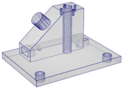
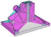
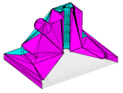
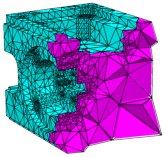
Figure 14: An input PLC (cami1a.poly, left), the generated Steiner CDT (middle, -p switch) in which Steiner points are located on the boundary edges of the PLC, and a constrained tetrahedralization (right, -pY switch) in which Steiner points lie in the interior of the PLC.
The default outputs of TetGen are four files listed in Table 6:
Other output switches are available by adding the switches: -f (output all faces including interior faces), -e (output all edges including interior edges), and -n (output the adjacency graph of the tetrahedra).
The -q switch adds new points to improve the mesh quality. It can be used together with -p (to refine a CDT), or -r (to refine a previously generated mesh), -a, or -m (to conform to a mesh sizing function).
TetGen enforces two quality constraints on tetrahedra: a maximum radius-edge ratio bound and a minimum dihedral angle bound. By default, these two constraints are 2.0 and 0 degrees, respectively. These quality constraints may be specified after the -q. The two constraints are separated by a slash ‘/’ (or ‘,’):
of any tetrahedron. For example, -q1.2 specifies a maximum radius-edge ratio of 1.2; -q1.2/10 specifies the same plus a minimum dihedral angle of 10 degrees. -q/7 specifies the default radius-edge ratio bound of 2 and a dihedral angle bound of 7 degrees.
For example, the following command uses the default quality constraints. It is equivalent to -pq2.0/0.
tetgen -pq thepart.smesh
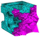
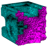
The screen output of the command line is shown below. Figure 15 illustrates three quality tetrahedral meshes of a PLC generated by applying different radius-edge ratio bounds.
Opening thepart.smesh.
Opening thepart.node.
Delaunizing vertices...
Delaunay seconds:  0.03408
Creating surface mesh ...
Surface mesh seconds:  0.004497
Constrained Delaunay...
Constrained Delaunay seconds:  0.025309
Removing exterior tetrahedra ...
Exterior tets removal seconds:  0.001419
Refining mesh...
Refinement seconds:  0.489247
Optimizing mesh...
Optimization seconds:  0.014569

Writing thepart.1.node.
Writing thepart.1.ele.
Writing thepart.1.face.
Writing thepart.1.edge.

Output seconds:  0.048593
Total running seconds:  0.618028

Statistics:

  Input points: 994
  Input facets: 1995
  Input segments: 1491
  Input holes: 0
  Input regions: 0

  Mesh points: 8029
  Mesh tetrahedra: 33773
  Mesh faces: 73092
  Mesh faces on facets: 11092
  Mesh edges on segments: 5143
  Steiner points inside domain: 2485
  Steiner points on facets:  898
  Steiner points on segments:  3652
TetGen supports several ways of generating adaptive tetrahedral meshes. They have been described already in Section 1.2.6.
The -a switch is used in mesh refinement, i.e., together with -q. It imposes a maximum volume constraint on all tetrahedra. If a number follows the -a, no tetrahedra is generated whose volume is larger than that number. See Figure 18 for an example.
TetGen also supports other constraints such as the constraint of maximum face area and the constraint of maximum edge length imposed on facets and segments of the PLC, respectively.
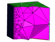
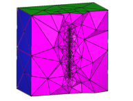
Figure 16 shows two examples of the results of applying constraints on a facet and a segment, respectively.
These constraints are imposed by using a .var file (Section 5.2.9).
The -m switch is used in mesh refinement, i.e., together with the -q switch. It applies a user-defined mesh sizing function which specifies the desired edge lengths in the final mesh. It aims to create an adaptive mesh whose edge lengths are conforming to this function. At the moment, only isotropic mesh sizing functions are supported.
TetGen assumes that the mesh sizing function is specified on a set of discrete points whose convex hull covers the mesh domain (i.e., the underlying space of the PLC). The mesh element size at any point in the domain is automatically computed by a linear interpolation from its adjacent points.
When the -m switch is used, TetGen will read a .mtr file, which stores the nodal mesh element size, i.e., the desired edge length at the location of the node in the mesh domain. There are two possible ways to specify the sizing function.
 .
.
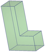
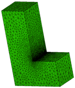
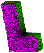
Figure 17: The tetrahedral meshes of a PLC (L.smesh) generated by the commands: -pqm. A sizing function (L.mtr) was applied on the nodes of the PLC. Both input files are found in Section 5.2.8.
The -r switch reconstructs an existing tetrahedral mesh. Usually, the purpose of using this switch is to refine the mesh to improve its quality, i.e., to use it together with the -q switch. Other usages of the -r switch are possible, such as inserting additional points (-i switch), mesh adaptation (-m switch), and linear function interpolation (-m switch plus a background mesh).
The -O switch specifies a mesh optimization level and chooses the operations. Both are integers and are separated by a slash ‘/’.
The mesh optimization level is an integer ranged from 0 to 10, where 0 means no mesh optimization is executed. The larger the level is, the more mesh optimization iterations will be performed, and TetGen may run very slow. Default the mesh optimization level is 2.
There are three local operations available in TetGen for optimizing the mesh, which are:
The integer for choosing operations is ranged from 0 to 7. Here 0 means no operation is chosen (hence no mesh optimization will be done). Each operation is enabled/disabled by setting the corresponding bit in this integer.
The default is 7, i.e., all of these three operations are enabled.
For examples, the switch -O2/7 specifies the optimization level 2 and uses all optimizing operations. These are the default switches in TetGen. The switch -O/1 chooses only the edge/face flip operation and uses the default optimization level.
The current objective function to be optimized by TetGen is to reduce the maximum dihedral angle of the tetrahedra. The default value is 165 degree. One can set this value after the -o/. For example, -o/150 sets the maximum dihedral angle to be 150 degree.
The -R switch indicates that some vertices of an existing tetrahedral mesh are to be removed. TetGen provides two ways to indicate those vertices to be removed.
The -R switch only removes vertices which can be removed. In particular, such vertices lie in the interior of the domain, or vertices lying in the interior of a facet or a segment. Note that this switch does not guarantee that all the marked vertices are successfully removed.
Once the mesh has been coarsened, the mesh quality may decrease. You may use the -q switch together with the -R switch. It will trigger the mesh improvement algorithm of TetGen to improve the mesh quality after the mesh coarsening.
The -i switch indicates that a list of additional points is going to be inserted into an existing tetrahedral mesh. The list of additional nodes is read from files xxx.a.node, where xxx stands for the input file name (i.e., xxx.poly or xxx.smesh, or xxx.ele, ...). This switch is useful for refining a finite element or finite volume mesh using a list of user-defined points.
The -A switch assigns an additional attribute (an integer number) to each tetrahedron that identifies to what facet-bounded region each tetrahedron belongs. In the output mesh, all tetrahedra in the same region will get a corresponding non-zero attribute.
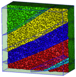
Figure 18 shows an example of tetrahedral meshes of a PLC which contains several sub-domains.
TetGen provides various switches to output its mesh. They are summarized below.
The -f switch outputs all triangular faces (including interior faces) of the mesh into a .face file. Without -f, only the boundary faces or the convex hull faces are output.
In the .face file, interior faces and boundary (or convex hull) faces are distinguished by their boundary markers. Each interior face has a boundary marker ‘0’. A non-zero boundary marker means a boundary or convex hull face.
The -e switch outputs all mesh edges (including interior edges) of the mesh into a .edge file. Without -e, only the boundary edges are output.
In the .edge file, interior edges and boundary edges are distinguished by their boundary markers. Each interior edge has a boundary marker ‘0’. A non-zero boundary marker means a boundary edge.
The -n switch outputs the neighboring tetrahedra to a .neigh file. Each tetrahedron has four neighbors. The first neighbor of this tetrahedron is opposite to the first of its corner, and so on. The neighbors are given by their indices in the corresponding .ele file. A ‘-1’ indicates that there is no neighbor at this face of the tetrahedron.
If the -nn switch is used, TetGen also outputs the neighboring tetrahedra to each face of the mesh in the corresponding .face file.
The -z switch numbers all output items starting from zero. This switch is useful in case of calling TetGen from another program.
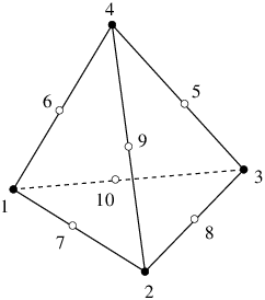
With the -o2 switch, TetGen will output the tetrahedral mesh with quadratic elements which have 10 nodes per tetrahedron, 6 nodes per triangular face, and 3 nodes per edge. The positions of these extra nodes in each element is shown in Figure 20.
The -V switch gives detailed information about what TetGen is doing. More ‘V’s are increasing the amount of detail.
Specifically, -V gives information on algorithmic progress and more detailed statistics including a rough mesh quality report. Below is a screen output of the quality report.
Mesh quality statistics:

  Smallest volume:         0.016741   |  Largest volume:           125.77
  Shortest edge:            0.30902   |  Longest edge:             12.189
  Smallest asp.ratio:        1.2927   |  Largest asp.ratio:        16.964
  Smallest facangle:         15.352   |  Largest facangle:       141.8279
  Smallest dihedral:          5.587   |  Largest dihedral:       163.9413

  Aspect ratio histogram:
         < 1.5       :         5      |      6 - 10         :        33
     1.5 - 2         :       105      |     10 - 15         :         4
       2 - 2.5       :       228      |     15 - 25         :         1
     2.5 - 3         :       215      |     25 - 50         :         0
       3 - 4         :       321      |     50 - 100        :         0
       4 - 6         :       150      |    100 -            :         0
  (A tetrahedron's aspect ratio is its longest edge length divided by its
    smallest side height)

  Face angle histogram:
      0 -  10 degrees:         0      |     90 - 100 degrees:       637
     10 -  20 degrees:       122      |    100 - 110 degrees:       131
     20 -  30 degrees:       556      |    110 - 120 degrees:       101
     30 -  40 degrees:       700      |    120 - 130 degrees:        44
     40 -  50 degrees:      1273      |    130 - 140 degrees:         5
     50 -  60 degrees:      1085      |    140 - 150 degrees:         1
     60 -  70 degrees:      1129      |    150 - 160 degrees:         0
     70 -  80 degrees:       871      |    160 - 170 degrees:         0
     80 -  90 degrees:       506      |    170 - 180 degrees:         0

  Dihedral angle histogram:
       0 -  5 degrees:         0      |     80 - 110 degrees:      1675
       5 - 10 degrees:        10      |    110 - 120 degrees:       228
      10 - 20 degrees:       141      |    120 - 130 degrees:       149
      20 - 30 degrees:       362      |    130 - 140 degrees:        92
      30 - 40 degrees:       487      |    140 - 150 degrees:        77
      40 - 50 degrees:       762      |    150 - 160 degrees:        32
      50 - 60 degrees:       770      |    160 - 170 degrees:         7
      60 - 70 degrees:       812      |    170 - 175 degrees:         0
      70 - 80 degrees:       768      |    175 - 180 degrees:         0
To get the statistics for an existing mesh, run TetGen on that mesh with the -rNEF switches to read the mesh and print the statistics without writing any file.
Moreover, -V also gives information on the memory usage of TetGen. Below is a screen output of the memory usage report.
Memory usage statistics:

  Maximum number of tetrahedra:  45309
  Maximum number of tet blocks (blocksize = 8188):  6
  Approximate memory for tetrahedral mesh (bytes):  8,920,640
  Approximate memory for extra pointers (bytes):  1,775,824
  Approximate memory for algorithms (bytes):  637,136
  Approximate memory for working arrays (bytes):  2,092,580
  Approximate total used memory (bytes):  13,426,180
-VV gives more details on the algorithms, and slows down the execution, while -VVV is only useful for debugging.
TetGen allocates memory in blocks. Each block is a chunk of memory allocated once. It stores a number of mesh entities, i.e., vertices, tetrahedra, boundary faces, and boundary edges. TetGen will dynamically allocate new blocks when they are needed.
By default, each block consists of 8188 tetrahedra. This data size may be too small for generating large meshes. This may slow down the performance of TetGen. The -x switch allows users to set the desired number of elements allocated in one block.
If the -V switch is used, TetGen will report its memory usage, see Section 4.2.11. A hint to enlarge the block size can be seen from the “Maximum number of tet blocks” (the second line in this report). If this number is large (for example 10000), it is reasonable to enlarge the block size.
The -c switch keeps the convex hull of the tetrahedral mesh. By default, TetGen removes all tetrahedra which do not lie in the interior of the PLC (the domain) which may have an arbitrary shape and topology, i.e., it may be non-convex and may contain holes. If the -c switch is used, tetrahedra in the exterior of the PLC are not removed. The union of the mesh elements is a topological ball.
TetGen assigns to all exterior tetrahedra a region attribute ‘-1’, so that they can be distinguished from the interior tetrahedra.
The -S switch specifies a maximum number of Steiner points (points that are not in the input) which are added by mesh refinement to improve the mesh quality. The default is to allow an unlimited number of Steiner points.
The -C switch indicates TetGen to check the consistency of the mesh on finish. If it is specified twice, i.e., -CC, TetGen also checks the constrained Delaunay (for the -p switch) or conforming Delaunay (for -q, -a, or -i) property of the mesh.
With the -I switch, TetGen does not use the iteration numbers. It suppresses the output of .node file, so your input file will not be overwritten. It cannot be used with the -r switch, because that would overwrite your input .ele file. It shouldn’t be used with the -q switch if one is using a .node file for input, because no .node file is written, so there is no record of any added Steiner points.
The -T switch sets a user-defined tolerance used by many computations of TetGen, default is 10−8.
In principle, the vertices which are used to define a facet of a PLC should be exactly coplanar. But this is very hard to achieve in practice due to the inconsistent nature of the floating-point format used in computers.
TetGen accepts facets whose vertices are not exactly but "approximately coplanar". Four points a, b, c and d are assumed to be coplanar as long as the ratio v / l3 is smaller than the given tolerance, where v and l are the volume and the average edge length of the tetrahedron abcd, respectively.
To choose a proper tolerance according to the input point set will usually reduce the number of adding points and improve the mesh quality.
Files are used as input and output when using TetGen as a stand-alone program. This section describes the input/output file formats of TetGen. When using TetGen as a library, the data structure tetgenio (explained in Section 6) is used to transfer the data stored in files.
In TetGen, a 3d PLC is described by a boundary discretization (e.g., a surface mesh) of the PLC. This description can be viewed as a Boundary Representation (B-Rep) without topological information, i.e., there are no information like incidences and orientations about edges and facets. This makes the description simple and it can describe non-manifolds easily. TetGen will recover and validate the topological information from this description during its meshing process.
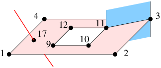
The boundary description of a PLC contains the set of vertices and facets of the PLC. Recall that each facet of a PLC is a 2d PLC. It may contain holes, segments and vertices in its interior, see Figure 19 for an example. TetGen describes a facet by a list of polygons and a list of holes. Each polygon of a facet is described by an ordered list of vertices. The order of the vertices can be in either clockwise or counterclockwise order. A polygon may be degenerate, i.e., it may contain only one or two vertices. A degenerate polygon is used to represent an isolated vertex or segment in this facet, see Fig. 19.
A hole in a facet is described by specifying an arbitrary point p ∈ ℝ3, such that the projection of p onto this facet lies strictly in the interior of this hole. Note that p is not a vertex of the PLC.
Remark. By the definition of a PLC, all vertices of a facet must lie in the same affine subspace of that facet. However, this requirement is generally impossible to be satisfied in practice due to the floating-point numbers used in computer. TetGen only requires that all vertices of a facet are approximately coplanar.
In addition, a list of holes and sub-regions of the PLC can be defined. A hole of the PLC is described by specifying an arbitrary point p ∈ ℝ3 that lies strictly in the interior of the hole. Sub-regions are described exactly the same way. Note that the points used to define holes and sub-regions are not vertices of the PLC.
This description of a PLC is further explained in the input file formats of TetGen, i.e., the .node, .poly, and .smesh file formats.
In TetGen, the mesh entities like vertices, edges, and faces, are assigned with a boundary marker. Boundary markers are tags (integers) used mainly to identify which entities are associated with which boundary element of the input PLC, such as, a segment or a facet. A common application is to determine where boundary conditions should be applied to a finite element mesh. You can prevent boundary markers from being written into files produced by TetGen by using the -B switch.
Mesh entities which are not on the boundary of the PLC must have the boundary markers ‘0’.
Mesh entities which are on the boundary will be assigned to a boundary marker that is the same as the boundary marker of that boundary of the PLC. However, if a boundary of a PLC does not have a boundary marker or have a marker ‘0’, TetGen will assign a ‘1’ to those entities belong to this boundary in the output files. This way, TetGen is able to distinguish them from other interior mesh entities.
Table 7 lists all file formats that are used by TetGen. All files are of ASCII form and may contain comments prefixed by the character ’#’. Points, tetrahedra, facets, edges, holes, and maximum volume constraints must be numbered consecutively, starting from either 1 or 0. However, all input files must be consistent. TetGen automatically detects your choice while reading the .node (or .poly or .smesh) file. When calling TetGen from another program, use the -z switch if you wish to number objects from zero.
.node input/output a list of nodes. .poly input a piecewise linear complex. .smesh input/output a piecewise linear complex. .ele input/output a list of tetrahedra. .face input/output a list of triangular faces. .edge input/output a list of edges. .vol input a list of maximum volumes. .mtr input/output a mesh sizing function. .var input a list of variant constraints. .neigh output a list of neighbors.
Table 7: Overview of TetGen’s file formats.
Remark: in the following description ‘#’ stands for ‘number’ – it should not cause confusion with the comment prefix.
A .node file contains a list of 3d points.
  First line:  <# of points> <dimension (3)> <# of attributes>
               <boundary markers (0 or 1)>
  Remaining lines list # of points:
    <point #> <x> <y> <z> [attributes] [boundary marker]
    ...
Each point has three coordinates (x, y and z), probably has one or several attributes, and a boundary marker as well. The .node files are used as both input and output files to represent the point set of a PLC, or the point set of a mesh, or the set of additional points (for the -i switch) which need to be inserted into a mesh. The example below demonstrates the layout of the .node file.
  # Node count, 3 dim, no attribute, no boundary marker
  8  3  0  0
  # Node index, node coordinates
  1  0.0 0.0 0.0
  2  1.0 0.0 0.0
  3  1.0 1.0 0.0
  4  0.0 1.0 0.0
  5  0.0 0.0 1.0
  6  1.0 0.0 1.0
  7  1.0 1.0 1.0
  8  0.0 1.0 1.0
The attributes, which are typically floating-point values of physical quantities (such as mass or conductivity) associated with the points, are copied unchanged to the output mesh.
If -p, -q, -a, or -i is selected, each Steiner point added to the mesh has attributes zero.
If the -w (weighted Delaunay tetrahedralization) switch is specified, the first attribute is regarded as the weight of that point.
If the <boundary marker> of the first line is 1, the last column of the remainder of the file is assumed to contain boundary markers. Boundary markers are used to identify boundary points (points resting on PLC facets). The .node file produced by TetGen contains boundary markers in the last column unless they are suppressed by the -B switch. The boundary marker associated with each point in an output .node file is chosen as follows:
TetGen can determine which points are on the boundary. Input with the boundary marker zero (or use no markers at all) will result in output with boundary marker 1 for all points on the boundary.
If the -R (mesh coarsening) switch is used, points with boundary markers equal to −1 will be removed.
A .poly file is a B-Rep description of a piecewise linear complex (PLC) containing some additional information. It consists of four parts.
The first three parts are mandatory, but the fourth part is optional. They are respectively described below.
Part 1 lists all the points, and is identical to the format of .node files. <# of points> may be set to zero to indicate that the points are listed in a separate .node file.
  First line:  <# of points> <dimension (3)> <# of attributes>
               <boundary markers (0 or 1)>
  Remaining lines list # of points:
    <point #> <x> <y> <z> [attributes] [boundary marker]
    ...
The facet list is given by
  One line: <# of facets> <boundary markers (0 or 1)>
  Following lines list # of facets:
     <facet #>
     ...
The format of a single facet is:
  One line: <# of polygons> [# of holes] [boundary marker]
  Following lines list # of polygons:
    <# of corners> <corner 1> <corner 2> ... <corner #>
    ...
  Following lines list # of holes:
    <hole #> <x> <y> <z>
    ...
Each facet is a polygonal region which may contain segments, single points and holes. It consists of a list of polygons. Each polygon is specified by giving the number of corners n, n ≥ 1, followed by the list of ordered indices of those corners. It does not matter which order (counterclockwise or clockwise) you choose to list the indices. It can be degenerate, i.e., n = 1 or n = 2 indicates a single point or a segment, respectively.
A hole in a facet is specified by identifying a point inside the hole. The list of hole points (consecutively) follows the list of polygons.
Boundary markers of facets are tags (integers) used mainly to identify which faces of the tetrahedralization are associated with which PLC facet, hence identify which faces occur on a boundary of the tetrahedralization. A common application is to use them to determine where different boundary condition types should be applied to a mesh.
If the [boundary marker] is 1, each facet is assumed to have a boundary marker (an integer). TetGen will produce an additional boundary marker for each face in the .face (output) file (in the last column of each record).
If the [boundary marker] is 0, TetGen will automatically assign a 1 to all boundary faces (which belong to facets of the PLC) in the .face (output) file.
You can prevent boundary markers from being written into the .face file by using the -B switch.
Note that each line of indices should not be arbitrarily long because the maximum characters per line read by TetGen is 1024. The list can be broken into several lines.
Holes in the volume are specified by identifying a point inside each hole.
  One line: <# of holes>
  Following lines list # of holes:
    <hole #> <x> <y> <z>
    ...
After the constrained Delaunay tetrahedralization is formed, TetGen creates holes by removing tetrahedra. This exactly is the reason that TetGen requires a closed boundary of the PLCs. In case of non-closed PLC facets the whole tetrahedralization will be “eaten" away. If two tetrahedra abutting a boundary face are removed, the boundary face itself is also vanished.
Hole points have to be placed inside a region, else the rounding error determines which side of the facet is being transformed into the hole.
The optional fourth section lists regional attributes (to be assigned to all tetrahedra in a region) and regional constraints on the maximum tetrahedron volume. TetGen will read this section only if the -A switch is used or the -a switch without a number is invoked. Regional attributes and volume constraints are propagated in the same manner as holes.
  One line: <# of region>
  Following lines list # of region attributes:
    <region #> <x> <y> <z> <region number> <region attribute>
    ...
If two values are written on a line after the x, y and z coordinate, the former is assumed to be a regional attribute (but will only be applied if the -A switch is selected), and the latter is assumed to be a regional volume constraint (but will only be applied if the -a switch is selected). It is possible to specify just one value after the coordinates. It can serve as both an attribute and a volume constraint, depending on the choice of switches. A negative maximum volume constraint allows to use the -A and the -a switches without imposing a volume constraint in this specific region.
In the following, a unit (1 × 1 × 1) cube is described by the poly file format.
  # Part 1 - node list
  # node count, 3 dim, no attribute, no boundary marker
  8  3  0  0
  # Node index, node coordinates
  1  0.0 0.0 0.0
  2  1.0 0.0 0.0
  3  1.0 1.0 0.0
  4  0.0 1.0 0.0
  5  0.0 0.0 1.0
  6  1.0 0.0 1.0
  7  1.0 1.0 1.0
  8  0.0 1.0 1.0

  # Part 2 - facet list
  # facet count, no boundary marker
  6  0
  # facets
  1            # 1 polygon, no hole, no boundary marker
  4  1 2 3 4   # front
  1
  4  5 6 7 8   # back
  1
  4  1 2 6 5   # bottom
  1
  4  2 3 7 6   # right
  1
  4  3 4 8 7   # top
  1
  4  4 1 5 8   # left

  # Part 3 - hole list
  0            # no hole

  # Part 4 - region list
  0            # no region
A .smesh file is also a B-Rep description of a PLC. It describes a simple B-Rep model where each of its facet only has exactly one polygon, no holes, no segment and no point inside. It is less flexible than the .poly file format, while it is much simpler and useful when the boundary of PLC consists of only simple polygons, i.e., triangles, quads, etc.
Analogously to the .poly file format, the .smesh file format consists of four parts, which are points, facets, holes and regions, respectively. Only the second part, which describes facets, is different. It is described below.
Each facet consists of exactly one polygon. The corner list of each polygon can be distributed over a number of lines. The optional boundary marker of each facet is given at the end of the corner list.
  One line: <# of facets> <boundary markers (0 or 1)>
  Following lines list # of facets:
    <# of corners> <corner 1> ... <corner #> [boundary marker]
    ...
The following example demonstrates the layout of the facet part of the unit cube.
  # Part 2 - facet list
  # facet count, no boundary marker
  6  0
  # facets
  4  1 2 3 4   # front
  4  5 6 7 8   # back
  4  1 2 6 5   # bottom
  4  2 3 7 6   # right
  4  3 4 8 7   # top
  4  4 1 5 8   # left
An .ele file contains a list of tetrahedra.
  First line: <# of tetrahedra> <nodes per tet. (4 or 10)>
              <region attribute (0 or 1)>
  Remaining lines list # of tetrahedra:
    <tetrahedron #> <node> <node> ... <node> [attribute]
    ...
Each tetrahedron has four corners (or ten corners if the -o2 switch is used). Nodes are indices into the corresponding .node file. The first four nodes are the corner vertices. If -o2 switch is used, the remaining six nodes are generated on the midpoints of the edges of the tetrahedron. Figure 20 shows how these corners and the second-order nodes are locally numbered. Second order nodes are output only. They are omitted by the mesh reconstruction (the -r switch).
If the <region attribute> in the first line is 1, each tetrahedra has an additional region attribute (an integer) in the last column. Region attributes of tetrahedra are tags used mainly to identify which tetrahedra of the tetrahedralization are associated with which facet-bounded region (sub-domain) of the PLC, set in the fourth part of a .poly or a .smesh file. Region attributes do not diffuse across facets, all tetrahedra in the same region have exactly the same region attribute. A common application of the region attribute is to determine which material a tetrahedron has.
The .ele file is the default output file of TetGen. However, it can be omitted by -E switch. If -r switch is used, TetGen reads a .ele file and reconstructs a tetrahedral mesh from it.
The following example illustrates the layout of a .ele file.
  154  4  0
      1       4   107     3    50
      2       4   108     3   107
      3       9    97    95    94
      4       4   107    50    93
      5      56     1    50    47
      6      94    98    97    95
      7      97     9    95    55
      ...
A .face file contains a list of triangular faces of the tetrahedralization.
  First line: <# of faces> <boundary marker (0 or 1)>
  Remaining lines list # of faces:
    <face #> <node> <node> <node> ... [boundary marker] ...
    ...
In its basic form, each face has three corners and possibly has a boundary marker. Nodes are indices of the corresponding .node file.
If the <boundary marker> in the first line is 1, each face has an additional boundary marker (an integer) in the last column. Boundary markers of facets are defined in the .poly or the .smesh files. The optional column of boundary markers can be suppressed by the -B switch.
If the -o2 switch is used, each face has three corners and three second-order nodes generated on the midpoints of the edges of this face. Figure 21 shows the local numbering of the corners and the second-order nodes of a face. They are listed after the corners of this face, and before its boundary marker. Second order nodes are output only. They are ignored during the mesh reconstruction (the -r switch).
If the -nn switch is used, each face contains two additional indices (after the boundary marker) in the corresponding .ele file. They are indices of the tetrahedra containing this face. A −1 indicates that there is no adjacent tetrahedron at this side, i.e., it is “outer space".
TetGen default only outputs the boundary faces or the convex hull faces into a .face file. If the -f switch is used, TetGen outputs all faces (including interior faces) of the tetrahedralization. In this case, each interior face will always have a ‘0’ as its boundary marker. This file can be omitted by using the -F switch.
If the -r switch is used, TetGen can also read the .face file for identifying boundary faces in a reconstructed mesh.
An .edge file contains a list of edges of the tetrahedralization.
  First line: <# of edges> <boundary marker (0 or 1)>
  Remaining lines list # of edges:
    <edge #> <endpoint> <endpoint> ... [boundary marker] ...
    ...
In its basic form, each edge has two endpoints and possibly a boundary marker (if the <boundary marker> in the first line is 1). Endpoints are indices in the corresponding .node file.
If the -o2 switch is used, each edge has a second order node (its midpoint). It is listed after its endpoints, and before its boundary marker. Second order nodes are output only. They are ignored during the mesh reconstruction (the -r switch).
If the -nn switch is used, each edge contains one additional index (after the [boundary marker]) in the corresponding .ele file. It is the index of a tetrahedron which contain this edge. A −1 indicates that there is no tetrahedron containing this edge.
If the -r switch is used, TetGen can also read the .edge file for identifying boundary edges in a reconstructed mesh.
The .edge file is the default output of TetGen when -p or -r switch is used. By default, it only contains a list of boundary edges (segments) of the tetrahedralization. If the -e switch is used, it contains a list of all edges (including interior edges) of the tetrahedralization. The output of this file can be suppressed by the -F switch.
A .vol file associates with each tetrahedron a maximum volume that is used for mesh refinement. It is read by TetGen in case the -r switch is used.
  First line: <# of tetrahedra>
  Remaining lines list # of maximum volumes:
    <tetrahedron #> <maximum volume>
    ...
As with other file formats, every tetrahedron must be represented, and they must be numbered consecutively. A tetrahedron may be left unconstrained by assigning it a zero or negative maximum volume to it.
The .mtr file assigns a mesh sizing function defined on the nodes of an input PLC, or an input tetrahedral mesh, or a background tetrahedral mesh. It is used when the -m switch is applied.
  First line: <# of nodes> <size of metric (always 1)>
  Remaining lines list # of point metrics:
    <value>
    ...
Each node is assigned a value that is interpreted by TetGen as the desired length for all edges connecting to the node. TetGen uses this size information to generate an adaptive tetrahedral mesh.
Below is an example of an L-shaped PLC (L.smesh) (see Figure 17):
# L.smesh
12  3  0  0
1  0 0 0
2  4 0 0
3  4 2 0
4  2 2 0
5  2 6 0
6  0 6 0
1  0 0 2
2  4 0 2
3  4 2 2
4  2 2 2
5  2 6 2
6  0 6 2
8  0
6  1 2 3 4 5 6
6  7 8 9 10 11 12
4  1 2 8 7
4  2 3 9 8
4  3 4 10 9
4  4 5 11 10
4  5 6 12 11
4  6 1 7 12
0
0
Below is an example file L.mtr to assign a sizing function on the nodes of the PLC:
# L.mtr
12  1
0.25
0.25
0.25
0.025
0.25
0.25
0.25
0.25
0.25
0.025
0.25
0.25
The following command generates the adaptive tetrahedral mesh shown in Figure 17.
tetgen -pqm L.smesh
It is possible to set a size 0 to a node. In this case, TetGen ignores the mesh element size at this node. For example, it is possible to use an L.mtr file like the following;
# L.mtr
12  1
0
0
0
0.025
0
0
0
0
0
0.025
0
0
A .var file allows you to specify maximum area constraints on facets and maximum length constraints on segments. They are used for mesh refinement.
  One line: <# of facet constraints>
  Remaining lines list # of facet constraints:
    <constraint #> <boundary marker> <maximum area>
    ...
  One line: <# of segment constraints>
  Remaining lines list # of segment constraints:
    <constraint #> <point1> <point2> <maximum length>
    ...
A constraint of maximum area on facet is set by specifying the boundary marker of that facet, which is the integer assigned to that facet in the corresponding .poly or .smesh file. A constraint of maximum length on segment is set by specifying the indices of the two endpoints of that segment.
Figure 16 shows two examples of the results of applying constraints on a facet and a segment, respectively.
A .neigh file associates with each tetrahedron its neighbors (adjacent tetrahedra), which are indices in the corresponding .ele file.
  First line:  <# of tetrahedra>  4
  Following lines list # of neighbors:
    <tetrahedra #> <neighbor> <neighbor> <neighbor> <neighbor>
    ...
An index of −1 indicates no neighbor (because the tetrahedron is on boundary of a mesh domain). The first neighbor of the tetrahedron i is opposite to the first corner of tetrahedron i, and so on. The .neigh file is output by TetGen when the -n switch is used.
A .v.node file contains a list of vertices of the Voronoi diagram or the power diagram ( -w switch). Each Voronoi vertex is the circumcenter (or the orthocenter) of a Delaunay (or weighted Delaunay) tetrahedron. The format of .v.node is the same as that of a .node file.
A .v.edge file contains a list of edges of the Voronoi diagram or the power diagram ( -w switch). Each edge corresponds to a face of the Delaunay (or weighted Delaunay) tetrahedralization.
Each Voronoi edge is either a line segment connecting two Voronoi vertices or a ray starting from a Voronoi vertex. The file format of a .v.edge file is
  First line:  <# of edges>
  Following lines list # of edges:
    <edge #> <vertex 1> <vertex 2> <V_x> <V_y> <V_z>
    ...
<vertex 1> and <vertex 2> are two indices pointing to the list of Voronoi vertices. <vertex 1> must be non-negative, while <vertex 2> may be −1 which means it is a ray. In this case, the unit vector of this ray is given by <V_x>, <V_y>, and <V_z>.
A .v.face file contains a list of faces of the Voronoi diagram or the power diagram ( -w switch). Each face corresponds to an edge of the Delaunay (or weighted Delaunay) tetrahedralization. It is formed by a list of Voronoi edges, which may not be closed. The file format of a .v.face file is
  First line:  <# of faces>
  Following lines list # of faces:
    <face #> <cell 1> <cell 2> <# of edges> <edge 1> <edge 2> ...
    ...
<cell 1> and <cell 2> are two indices pointing into the list of Voronoi cells, i.e., the two cells share this face. <edge 1>, <edge 2> ..., are indices pointing into the edge list, i.e., they are the edges of this face, there are total <# of edges>. If the face is not closed, the index of the last edge of this face is −1.
A .v.cell file contains a list of cells of the Voronoi diagram or the power diagram ( -w switch). Each cell corresponds to a vertex of the Delaunay (or weighted Delaunay) tetrahedralization. A cell is formed by a list of Voronoi faces, which may not be closed. The file format of a .v.cell file is
  First line:  <# of cells>
  Following lines list # of cells:
    <cell #> <# of faces> <face 1> <face 2> ...
    ...
<face 1>, <face 2>, ... are indices pointing into the Voronoi face list. There are total <# of faces> faces. If the cell is not closed, the index of the last face in this cell is −1.
TetGen supports additional polyhedral file formats as well. Table 8 lists the supported file formats. TetGen recognizes the file formats by the file extensions.
.off input Geomview’s polyhedral file format. .ply input Polyhedral file format. .stl input Stereolithography format. .mesh input/output Medit’s mesh file format.
Table 8: Overview of supported file formats.
The .off is the one of the file formats of Geomview http://www.geomview.org - an interactive 3d viewing program for Unix/Linux. It represents collections of planar polygons with possibly shared vertices, a convenient way to describe polyhedra. The polygons may be concave, but there’s no provision for polygons containing holes.
The full description of the .off file format can be found elsewhere on the internet. Below is a simple description of this file format.
OFF numVertices numFaces numEdges
 x y z
 x y z
 ... numVertices like above
 NVertices v1 v2 v3 ... vN
 MVertices v1 v2 v3 ... vM
 ... numFaces like above
Note that vertices are numbered starting at 0 (not starting at 1), and that numEdges will always be zero.
The .ply file format is a simple object description that was designed as a convenient format for researchers who work with polygonal models. Early versions of this file format were used at Stanford University and at UNC Chapel Hill.
A description examples as well as codes of the PLY file format can be found at http://paulbourke.net/dataformats/ply/.
The .stl or stereolithography format is an ASCII or binary file used in manufacturing. It is a list of the triangular surfaces that describe a computer generated solid model. This is the standard input for most rapid prototyping machines.
The description of the .stl file format can be found elsewhere on the web. An elaborated description can be found at http://en.wikipedia.org/wiki/STL_(file_format). Below is an example.
solid
 ...

 facet normal 0.00 0.00 1.00
    outer loop
      vertex  2.00  2.00  0.00
      vertex -1.00  1.00  0.00
      vertex  0.00 -1.00  0.00
    endloop
  endfacet
 ...
 endsolid
The .mesh is the file formats of Medit - an interactive 3d mesh viewing program http://www.ann.jussieu.fr/frey/software.html. This file format is described in the documentation of Medit.
A repository of free 3d models in this file format are available at INRIA’s Free 3d Meshes Download http://www-roc.inria.fr/gamma/gamma/Accueil/.
This section provides three examples. They are designed to support interactive learning. The topics are describing PLCs using TetGen’s .poly file format and constructing different quality meshes through the command line switches.
Figure 22 shows the geometry of a rectangular bar. This bar consists of eight nodes and six facets (which are all rectangles). In addition, there are two boundary markers (−1 and −2) associated to the leftmost facet and the rightmost facet, respectively. This simple model has its physical meaning. It can be seen as the geometry of a typical heat transfer problem. The task is to compute the temperature diffusion in the bar, in which the flow of heat moves from the hot side to the cold side. The two boundary markers can represent two different boundary conditions, one has high temperature and the other has low temperature. Here is the input file bar.poly describing the bar:
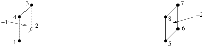
Figure 22: A bar having two boundary markers (−1 and −2) defined.
# Part 1 - the node list.
# A bar with 8 nodes in 3d, no attributes, no boundary marker.
8  3  0  0
  # The 4 leftmost nodes:
  1  0  0  0
  2  2  0  0
  3  2  2  0
  4  0  2  0
  # The 4 rightmost nodes:
  5  0  0  12
  6  2  0  12
  7  2  2  12
  8  0  2  12
# Part 2 - the facet list.
# Six facets with boundary markers.
6  1
  # The leftmost facet.
  1  0  -1   # 1 polygon, no hole, boundary marker (-1)
  4  1 2 3 4
  # The rightmost facet.
  1  0  -2   # 1 polygon, no hole, boundary marker (-2)
  4  5 6 7 8
  # Other facets.
  1
  4  1 5 6 2 # bottom side
  1
  4  2 6 7 3 # back side
  1
  4  3 7 8 4 # top side
  1
  4  4 8 5 1 # front side
# Part 3 - the hole list.
# There is no hole in bar.
0
# Part 4 - the region list.
# There is no region defined.
0
The command line is chosen as follows: first mesh the PLC (-p), then impose the quality constraint (-q). This will result in a quality mesh of four files: bar.1.node, bar.1.ele, bar.1.face, and bar.1.edge.
> tetgen -pq bar.poly
Here is the output file bar.1.node. It contains 47 points. The additional points were added by TetGen automatically to meet the quality measure.
47  3  0  0
   1    0  0  0
   2    2  0  0
   3    2  2  0
   4    0  2  0
   5    0  0  12
   6    2  0  12
   7    2  2  12
   8    0  2  12
   9    1.0000469999999999  0  0
  10    0  0.999668  0
  11    0  0.99944500000000003  12
  12    1.000594  0  12
  ...
# Generated by tetgen -pq bar.poly
Here is the output file bar.1.ele, which contains 83 tetrahedra.
83  4  0
    1      18    33    20    34
    2       9     2     3    25
    3      17    18    20    34
    4      43    32    18    37
    5      19    20    30    33
    6      14    41    13    42
    7      12    26     7     6
    8      10    28     1     9
    9      28    33    18    34
   10      35    41    38    45
   11      10     9    25    28
   12       3    25    19    30
   ...
# Generated by tetgen -pq bar.poly
Here is the output file bar.1.face with 90 boundary faces. Faces 1 and 2 are on the leftmost facet thus have markers −1; faces 3 and 4 have markers −2 indicating they are on the rightmost facet. Other faces have the default markers zero.
90  1
    1      3     4    10    -1
    2     10     9     3    -1
    3      7    12    11    -2
    4      7    11     8    -2
    5     18    37    43    0
    6     24    46    39    0
    7     26     6     7    0
    8     35    22    24    0
    9     29     7     8    0
   10     39     7    29    0
   11     29    11    27    0
   12     23    45    38    0
   ...
# Generated by tetgen -pq bar.poly
However, the mesh above may be too coarse for numerical simulation using finite element method or finite volume method. Using either the -q or the -a switch or both of them will result in a more dense quality mesh:
> tetgen -pq1.414a0.1 bar.poly
TetGen generates a mesh with 330 points and 1092 tetrahedra. The added points are due to both the -q and -a switches we have applied. To see a quality report of the mesh, type:
> tetgen -rNEFV bar.1.ele
In this example, we add an internal facet into the bar (in Figure 22), so that two sub-regions (separated by the newly added facet) in the bar are created. Figure 23 shows the modified geometry. This bar consists of twelve nodes (which I numbered) and seven facets (Note, some of them are not a single polygon any more). In addition, there are two regions defined, which have region attributes −10 and −20, respectively. Physically, you can associate two different materials to each of these two regions, and the two boundary markers (−1 and −2) in the last example still remain. Here is the input file bar2.poly describing the modified bar:
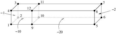
Figure 23: A bar having two regions (with region attributes −10 and −20, respectively) and two boundary markers (−1 and −2) defined.
# Part 1 - the node list.
# The model has 12 nodes in 3d, no attributes, no boundary marker.
12  3  0  0
  # The 4 leftmost nodes:
  1  0  0  0
  2  2  0  0
  3  2  2  0
  4  0  2  0
  # The 4 rightmost nodes:
  5  0  0  12
  6  2  0  12
  7  2  2  12
  8  0  2  12
  # The 4 added nodes:
  9  0  0  3
  10 2  0  3
  11 2  2  3
  12 0  2  3
# Part 2 - the facet list.
# Seven facets with boundary markers.
7  1
  # The leftmost facet.
  1  0  -1   # 1 polygon, no hole, boundary marker (-1)
  4  1 2 3 4
  # The rightmost facet.
  1  0  -2   # 1 polygon, no hole, boundary marker (-2)
  4  5 6 7 8
  # Each of following facets has two polygons, which are
  # one rectangle (6 corners) and one segment.
  2
  6  1 9 5 6 10 2 # bottom side
  2  9 10
  2
  6  2 10 6 7 11 3 # back side
  2  10 11
  2
  6  3 11 7 8 12 4 # top side
  2  11 12
  2
  6  4 12 8 5 9 1 # front side
  2  12 9
  # The internal facet separates two regions.
  1
  4  9 10 11 12
# Part 3 - the hole list.
# There is no hole in bar.
0
# Part 4 - the region list.
# There are two regions (-10 and -20) defined.
2
  1  1.0 1.0 1.5  -10  0.1
  2  1.0 1.0 5.0  -20  -1
The command line tetgen -pqaA bar2.poly generates the file bar2.1.ele. The first eight lines are listed next. It differs from bar.1.ele in that each record has an additional region attribute.
431  4  1
    1      32    57    50    60    -20
    2      51    23    50    49    -20
    3      88   138   116   149    -10
    4      76    96    95    36    -20
    5      29    55    56    52    -20
    6     132   138    88   139    -10
    7      65   138   132   139    -10
    8      16    54    53    15    -20
    ...
# Generated by tetgen -pqaA bar2.poly
Visualization of the resulting meshes (by TetView or other tools) shows that the refinement in the region with attribute −10 is denser than in that with −20. This is due to the volume constraints, (0.1) defined in the file bar2.poly, and due to the -aA switches.
This is the example file (example.poly) coming together with the TetGen’s source distribution. The geometry as well as some generated mesh are shown in Figure 24.
# Part 1 - the node list.
28  3  0  1
1  0  0  0  1
2  2  0  0  1
3  2  2  0  1
4  0  2  0  1
5  0  0  4  9
6  2  0  4  9
7  2  2  3  9
8  0  2  3  9
9  0  0  5  2
10  2  0  5  2
11  2  2  5  2
12  0  2  5  2
13  0.25  0.25  0.5  4
14  1.75  0.25  0.5  4
15  1.75  1.5  0.5  4
16  0.25  1.5  0.5  4
17  0.25  0.25  1  4
18  1.75  0.25  1  4
19  1.75  1.5  1  4
20  0.25  1.5  1  4
21  0.25  0  2  4
22  1.75  0  2  4
23  1.75  1.5  2  4
24  0.25  1.5  2  4
25  0.25  0  2.5  4
26  1.75  0  2.5  4
27  1.75  1.5  2.5  4
28  0.25  1.5  2.5  4
# Part 2 - the facet list
23  1
1  0  1  # 1
4    1  2  3  4
1  0  9  # 2
4    5  6  7  8
2  1  3  # 3
4    1  2  6  5
4    21  22  26  25
1  1  0  2.25
1  0  3  # 4
4    2  3  7  6
1  0  3  # 5
4    3  4  8  7
1  0  3  # 6
4    4  1  5  8
1  0  2  # 7
4    9  10  11  12
1  0  3  # 8
4    9  10  6  5
1  0  3  # 9
4    10  11  7  6
1  0  3  # 10
4    11  12  8  7
1  0  3  # 11
4    12  9  5  8
1  0  4  # 12
4    13  14  15  16
1  0  4  # 13
4    17  18  19  20
1  0  4  # 14
4    13  14  18  17
1  0  4  # 15
4    14  15  19  18
1  0  4  # 16
4    15  16  20  19
1  0  4  # 17
4    16  13  17  20
1  0  4  # 18
4    21  22  23  24
1  0  4  # 19
4    25  26  27  28
1  0  4  # 20
4    21  22  26  25
1  0  4  # 21
4    22  23  27  26
1  0  4  # 22
4    23  24  28  27
1  0  4  # 23
4    24  21  25  28
# Part 3 - the hole list
2
1  1  0.4  2.25
2  1  0.4  0.75
# Part 4 - the region list
2
1  1  0.25  0.1  10  0.001
2  1  0.5  4  20  0.01
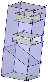
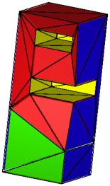
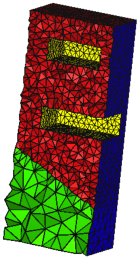
Figure 24: Left: A PLC with two sub-regions (materials) and two holes. Middle: the CDT generated by the command line: -pA. Right: The quality tetrahedral mesh generated by the command line: -pqAa.
One can use TetGen as a library so that it can be called directly from another program. This section gives the necessary instructions for using the TetGen library. Users are supposed to be able to use TetGen, i.e., know its command line switches and the input and output file formats. We refer to Section 3 for the instructions of how to compile TetGen into a library.
Programs calling TetGen must include the header file tetgen.h.
#include "tetgen.h"
It includes all data types and function declarations of the TetGen library. It defines the function tetrahedralize() and the data type tetgenio, which are provided for users to call TetGen with all its functionality. They are described in Section 6.2 and Section 6.3, respectively.
The function tetrahedralize() is declared as follows:
void tetrahedralize(char *switches, tetgenio *in, tetgenio *out,
                    tetgenio *addin = NULL, tetgenio *bgmin = NULL);
The parameter switches is a string containing the command line switches for this call. In this string, no initial dash ’-’ is required. The Q (quiet) switch is recommended in the final code. Some file output switches, like I and g are ignored.
The parameters in and out, which are two pointers pointing to objects of tetgenio, describing the input and the output. in and out must not be NULL.
Two additional parameters addin and bgmin may be supplied. When the switch -i is used, addin contains a list of additional vertices to be inserted. When the switch -m is used, bgmin contains a background mesh which is used to provide a mesh sizing function.
The tetgenio structure is used to pass data into and out of the tetrahedralize() procedure. It replaces the input and output files of TetGen by a collection of arrays, which are used to store points, tetrahedra, boundary markers, and so forth. It is a C++ class including data fields and functions. The data fields of tetgenio:
    int firstnumber; // 0 or 1, default 0.
    int mesh_dim;    // must be 3.

    REAL *pointlist;
    REAL *pointattributelist;
    REAL *pointmtrlist;
    int *pointmarkerlist;
    int numberofpoints;
    int numberofpointattributes;
    int numberofpointmtrs;

    int *tetrahedronlist;
    REAL *tetrahedronattributelist;
    REAL *tetrahedronvolumelist;
    int *neighborlist;
    int numberoftetrahedra;
    int numberofcorners;
    int numberoftetrahedronattributes;

    facet *facetlist;
    int *facetmarkerlist;
    int numberoffacets;

    REAL *holelist;
    int numberofholes;

    REAL *regionlist;
    int numberofregions;

    REAL *facetconstraintlist;
    int numberoffacetconstraints;

    REAL *segmentconstraintlist;
    int numberofsegmentconstraints;

    int *trifacelist;
    int *trifacemarkerlist;
    int numberoftrifaces;

    int *edgelist;
    int *edgemarkerlist;
    int numberofedges;
In all cases, the first item in any array is stored starting at index [0]. However, that item is item number firstnumber (0 or 1) unless the z switch is used, in which case it is item number ‘0’. Now the description of arrays follows.
An array of point coordinates. The first point’s x coordinate is at index [0], its y coordinate at index [1], and its z coordinate at index [2], followed by the coordinates of the remaining points. Each point occupies three REALs.
An array of point attributes. Each point’s attributes occupy numberofpointattributes REALs.
An array of point markers; one int per point.
An array of metric tensors at points. Each point’s tensor occupies numberofpointmtrs REALs.
An array of tetrahedron corners. The first tetrahedron’s first corner is at index [0], followed by its other three corners, followed by any other nodes if the ’-o2’ switch is used. Each tetrahedron occupies numberofcorners (4 or 10) ints.
An array of tetrahedron attributes. Each tetrahedron’s attributes occupy numberoftetrahedronattributes REALs.
An array of tetrahedron volume constraints; one REAL per tetrahedron. Input only.
An array of tetrahedron neighbors; four ints per tetrahedron. Output only.
An array of PLC facets. Each facet is an object of type facet (see Section 6.4.2).
An array of facet markers; one int per facet.
An array of holes. The first hole’s x, y and z coordinates are at indices [0], [1] and [2], followed by the remaining holes. Three REALs per hole.
An array of regional attributes and volume constraints. The first constraints’ x, y and z coordinates are at indices [0], [1] and [2], followed by the regional attribute at index [3], followed by the maximum volume at index [4], followed by the remaining volume constraints. Five REALs per volume constraint. Each regional attribute is used only if the A switch is used, and each volume constraint is used only if the a switch (with no number following) is used, but omitting one of these switches does not change the memory layout.
An array of facet maximum area constraints. Two REALs per constraint. The first one is the facet marker (cast the type to integer), the second is its maximum area bound. Note the ’facetconstraintlist’ is used only for the ’q’ switch.
An array of segment length constraints. Two REALs per constraint. The first one is the index (pointing into pointlist) of the node, the second is its maximum length bound. Note the ’segmentconstraintlist’ is used only for the ’q’ switch.
An array of triangular faces. The first face’s corners are at indices [0], [1] and [2], followed by the remaining faces. Three ints per face.
An array of face markers; one int per face.
An array of segment endpoints. The first segment’s endpoints are at indices [0] and [1], followed by the remaining segments. Two ints per segment.
An array of segment markers; one int per segment.
Two routines defined in tetgenio are used for memory initialization and cleaning. They are:
    void initialize();
    void deinitialize();
initialize() initializes all fields, that is, all pointers to arrays are initialized to NULL, and other variables are initialized to zero except the variable ’numberofcorners’, which is 4 (a tetrahedron has 4 nodes). Initialization is implicitly called by the constructor of tetgenio. For an example, the following line creates an object of tetgenio named io, all fields of io are initialized:
tetgenio io;
The next step is to allocate memory for each array which will be used. In C++ the memory allocation and deletion can be done by the new and delete operators. Another pair of functions (preferred by C programmers) are malloc() and free(). Whatever you use, you must stick with one of these two pairs, e.g., ’new’/’delete’ and ’malloc’/’free’ cannot be mixed. For example, the following line allocates memory for io.pointlist:
io.pointlist = new REAL[io.numberofpoints * 3];
deinitialize() frees the memory allocated in objects of tetgenio by using ’delete’. It is automatically called on deletion of the tetgenio objects. If the memory was allocated by using the function malloc(), the user is responsible to free it. After having freed all memory, one call of initialize() disables the automatic memory deletion.
To reuse an object is possible: first call deinitialize(), then call initialize() before the next use.
The facet data structure defined in tetgenio can be used to represent any facet of a PLC. The structure of facet shown below consists of a list of polygons and a list of hole points.
    typedef struct {
      polygon *polygonlist;
      int numberofpolygons;
      REAL *holelist;
      int numberofholes;
    } facet;
A polygon is again an object of type polygon. It consists of a list of corner points (vertexlist). The structure is shown below.
    typedef struct {
      int *vertexlist;
      int numberofvertices;
    } polygon;
The structure of a facet corresponds to the facet description in a .poly file format, described in Section 5.2.2. The front facet of Figure 23 serves an example for setting a PLC facet into an object of facet. It has two polygons, one has six vertices, and the other is a segment, no holes, the ASCII data is:
    2
    6  4 12 8 5 9 1 # front side
    2  12 9
The following C++ code does the translation. Assume the object of tetgenio is io and has already be created.
    tetgenio::facet *f;   // Define a pointer of facet.
    tetgenio::polygon *p; // Define a pointer of polygon.

    // All indices start from 1.
    io.firstnumber = 1;

    ...

    // Use 'f' to point to a facet of 'facetlist'.
    f = &io.facetlist[i];
    // Initialize the fields of this facet.
    //   There are two polygons, no holes.
    f->numberofpolygons = 2;
    // Allocate memory for polygons.
    f->polygonlist = new tetgenio::polygon[2];
    f->numberofholes = 0;
    f->holelist = NULL;

    // Set the data of the first polygon into facet.
    p = &f->polygonlist[0];
    p->numberofvertices = 6;
    // Allocate memory for vertices.
    p->vertexlist = new int[6];
    p->vertexlist[0] = 4;
    p->vertexlist[1] = 12;
    p->vertexlist[2] = 8;
    p->vertexlist[3] = 5;
    p->vertexlist[4] = 9;
    p->vertexlist[5] = 1;

    // Set the data of the second polygon into facet.
    p = &f->polygonlist[1];
    p->numberofvertices = 2;
    p->vertexlist = new int[2]; // Alloc. memory for vertices.
    p->vertexlist[0] = 12;
    p->vertexlist[1] = 9;
This section gives an example of how to call TetGen from another program by using the tetgenio data structure and the function tetrahedralize(). The input PLC in Section 5.4.1 (Figure 22) is used again.
The complete C++ source code is given below. It is also available on TetGen’s website:http://www.tetgen.org/files/tetcall.cxx. The code illustrates the following basic steps:
In addition, it outputs the PLC in the object in into two files (barin.node and barin.poly), and outputs the mesh in the object out into three files (barout.node, barout.ele, and barout.face).
This example can be compiled into an executable program.
g++ -o test tetcall.cxx -L./ -ltet
which will result an executable file test.
The complete source codes are given below:
#include "tetgen.h" // Defined tetgenio, tetrahedralize().

int main(int argc, char *argv[])
{
  tetgenio in, out;
  tetgenio::facet *f;
  tetgenio::polygon *p;
  int i;

  // All indices start from 1.
  in.firstnumber = 1;

  in.numberofpoints = 8;
  in.pointlist = new REAL[in.numberofpoints * 3];
  in.pointlist[0]  = 0;  // node 1.
  in.pointlist[1]  = 0;
  in.pointlist[2]  = 0;
  in.pointlist[3]  = 2;  // node 2.
  in.pointlist[4]  = 0;
  in.pointlist[5]  = 0;
  in.pointlist[6]  = 2;  // node 3.
  in.pointlist[7]  = 2;
  in.pointlist[8]  = 0;
  in.pointlist[9]  = 0;  // node 4.
  in.pointlist[10] = 2;
  in.pointlist[11] = 0;
  // Set node 5, 6, 7, 8.
  for (i = 4; i < 8; i++) {
    in.pointlist[i * 3]     = in.pointlist[(i - 4) * 3];
    in.pointlist[i * 3 + 1] = in.pointlist[(i - 4) * 3 + 1];
    in.pointlist[i * 3 + 2] = 12;
  }

  in.numberoffacets = 6;
  in.facetlist = new tetgenio::facet[in.numberoffacets];
  in.facetmarkerlist = new int[in.numberoffacets];

  // Facet 1. The leftmost facet.
  f = &in.facetlist[0];
  f->numberofpolygons = 1;
  f->polygonlist = new tetgenio::polygon[f->numberofpolygons];
  f->numberofholes = 0;
  f->holelist = NULL;
  p = &f->polygonlist[0];
  p->numberofvertices = 4;
  p->vertexlist = new int[p->numberofvertices];
  p->vertexlist[0] = 1;
  p->vertexlist[1] = 2;
  p->vertexlist[2] = 3;
  p->vertexlist[3] = 4;

  // Facet 2. The rightmost facet.
  f = &in.facetlist[1];
  f->numberofpolygons = 1;
  f->polygonlist = new tetgenio::polygon[f->numberofpolygons];
  f->numberofholes = 0;
  f->holelist = NULL;
  p = &f->polygonlist[0];
  p->numberofvertices = 4;
  p->vertexlist = new int[p->numberofvertices];
  p->vertexlist[0] = 5;
  p->vertexlist[1] = 6;
  p->vertexlist[2] = 7;
  p->vertexlist[3] = 8;

  // Facet 3. The bottom facet.
  f = &in.facetlist[2];
  f->numberofpolygons = 1;
  f->polygonlist = new tetgenio::polygon[f->numberofpolygons];
  f->numberofholes = 0;
  f->holelist = NULL;
  p = &f->polygonlist[0];
  p->numberofvertices = 4;
  p->vertexlist = new int[p->numberofvertices];
  p->vertexlist[0] = 1;
  p->vertexlist[1] = 5;
  p->vertexlist[2] = 6;
  p->vertexlist[3] = 2;

  // Facet 4. The back facet.
  f = &in.facetlist[3];
  f->numberofpolygons = 1;
  f->polygonlist = new tetgenio::polygon[f->numberofpolygons];
  f->numberofholes = 0;
  f->holelist = NULL;
  p = &f->polygonlist[0];
  p->numberofvertices = 4;
  p->vertexlist = new int[p->numberofvertices];
  p->vertexlist[0] = 2;
  p->vertexlist[1] = 6;
  p->vertexlist[2] = 7;
  p->vertexlist[3] = 3;

  // Facet 5. The top facet.
  f = &in.facetlist[4];
  f->numberofpolygons = 1;
  f->polygonlist = new tetgenio::polygon[f->numberofpolygons];
  f->numberofholes = 0;
  f->holelist = NULL;
  p = &f->polygonlist[0];
  p->numberofvertices = 4;
  p->vertexlist = new int[p->numberofvertices];
  p->vertexlist[0] = 3;
  p->vertexlist[1] = 7;
  p->vertexlist[2] = 8;
  p->vertexlist[3] = 4;

  // Facet 6. The front facet.
  f = &in.facetlist[5];
  f->numberofpolygons = 1;
  f->polygonlist = new tetgenio::polygon[f->numberofpolygons];
  f->numberofholes = 0;
  f->holelist = NULL;
  p = &f->polygonlist[0];
  p->numberofvertices = 4;
  p->vertexlist = new int[p->numberofvertices];
  p->vertexlist[0] = 4;
  p->vertexlist[1] = 8;
  p->vertexlist[2] = 5;
  p->vertexlist[3] = 1;

  // Set 'in.facetmarkerlist'

  in.facetmarkerlist[0] = -1;
  in.facetmarkerlist[1] = -2;
  in.facetmarkerlist[2] = 0;
  in.facetmarkerlist[3] = 0;
  in.facetmarkerlist[4] = 0;
  in.facetmarkerlist[5] = 0;

  // Output the PLC to files 'barin.node' and 'barin.poly'.
  in.save_nodes("barin");
  in.save_poly("barin");

  // Tetrahedralize the PLC. Switches are chosen to read a PLC (p),
  //   do quality mesh generation (q) with a specified quality bound
  //   (1.414), and apply a maximum volume constraint (a0.1).

  tetrahedralize("pq1.414a0.1", &in, &out);

  // Output mesh to files 'barout.node', 'barout.ele' and 'barout.face'.
  out.save_nodes("barout");
  out.save_elements("barout");
  out.save_faces("barout");

  return 0;
}
This section gives simplified explanations of some basic notions of combinatorial topology as a quick reference.
(a) (b) (c)
Figure 25: (a) A two-dimensional simplicial complex K consists of 2 triangles(which are shaded), 7 edges, and 5 vertices. (b) The underlying space. (c) A subcomplex, which is a 1-dimensional simplicial complex, consists of 4 edges, and 4 vertices.
A point set V ⊂ ℝd is convex if it contains every line segment whose end points are in this set. There are infinitely many convex sets containing V. The smallest convex set containing V is called the convex hull of V, denoted as convV. The dimension of the convex hull of V is the dimension of the affine space of V.
A simplex σ is the convex hull of an affinely independent set S of points. The dimension of σ is one less than the number of points of S. Specifically, in ℝ3 the maximum number of affinely independent points is 4, so we have non-empty simplices of dimensions 0, 1, 2 and 3 referred to as vertices, edges, triangles, and tetrahedra, respectively. For any subset T ⊆ S, the simplex τ = convT is a face of σ and we write τ ≤ σ. τ is a proper face of σ if T is a proper subset of S.
A simplicial complex K is a finite set of simplices such that (i) any face of a simplex in K is also in K, and (ii) the intersection of any two simplices in K is a face of both. Condition (ii) allows for the case in which two simplices are disjoint because the empty set is the unique (-1)-dimensional simplex, which is a face of any simplex. Figure 25 (a) illustrates a two-dimensional simplicial complex.
The underlying space of a set of simplices L, denoted |L|, is the union of simplices, ∪σ ∈ Lσ (see an illustration in Figure 25 (b)). |L| is a topologically closed set if and only if L is a simplicial complex.
A subcomplex of K is a subset of simplices of K that is also a simplicial complex. For an example see Figure 25 (c).
Convex polyhedra and their faces are well defined objects. It is a central topic in discrete geometry to study their structures and properties, see [29]. However, general polyhedra which are not necessarily convex are much complex objects. There exist various definitions in the literature. We adopt the definitions given by Edelsbrunner [7].
A polyhedron P is the union of convex polyhedra and the space of P is connected. It is not necessarily convex, see Figure 26 left for an example. The dimension of P is the dimension of the smallest affine space that contains P. The interior of P, denoted as int(P) is the point set such that every point p ∈ int(P) has a neighborhood (e.g., an open ball centered at this point) which is a subset of P. The boundary of P is the point set bd(P) = P − int(P).
A face F of P satisfies the following three conditions:
F is also a polyhedron whose dimension is the dimension of the affine space that determines F. 0-, 1-, and 2-dimensional faces of P are called vertices, edges, and facets of P. Each facet is a polygonal region which may not be convex and may contain holes in it, as illustrated in the right of Figure 26.
In geometric and solid modeling, constructive solid geometry (CSG) and boundary representation (B-Rep) are two popular representations for three-dimensional objects.
A CSG model implicitly describes the domain as a combination of simple primitives or other solids in a series of Boolean operations. It can describe rather complicated shapes simply. However, the domain boundary must be calculated numerically in order to find the intersecting points, curves, and patches. This involves solving many non-linear equations in three variables. Obtaining a PLC from a CSG model is generally not a simple task.
A B-Rep model explicitly describes the domain boundary by a set of non-overlapping facets (may be curved surfaces) together with topological information (such as incidence and adjacency) between the facets. The volume of the domain is implicitly bounded by them. However, it is not trivial to correctly define such a model for a complex object. Nevertheless, The B-Rep model is popularly used in describing 3d geometries.
The list of error codes and messages can also be found in the function terminatetetgen() defined in the file tetgen.h.
code 1 message Error: Out of memory
code 2 message Please report this bug to Hang.Si@wias-berlin.de. Include the message above, your input data set, and the exact command line you used to run this program, thank you description This failure was caused by a known bug of TetGen.
code 3 message A self-intersection was detected. Program stopped. Hint: use -d option to detect all self-intersections. description This failure was caused by an input error.
code 4 message A very small input feature size was detected. Program stopped. Hint: use -T option to set a smaller tolerance. description This failure was caused by a possible input error. For example, there are two segments nearly intersecting each. other. If you want to ignore this possible error, set a smaller tolerance by the -T switch, default is 10−8.
code 5 message Two very close input facets were detected. Program stopped. Hint: use -Y option to avoid adding Steiner points on boundary. description This failure was caused by a possible input error. For example, there are two facets nearly overlapping each other. Once Steiner points are added to one of the facets, it will cause a self-intersection.
code 10 message An input error was detected. Program stopped. description This failure was caused by an input error.
|
|
This document was translated from LATEX by HEVEA.