TetGen is a robust, fast, and easy-to-use software for generating tetrahedral meshes suitable in many applications.
For a set of 3d (weighted) points, TetGen generates the Delaunay and weighted Delaunay tetrahedralization as well as their duals, the Voronoi diagram and power diagram. For a 3d polyhedral domain, TetGen generates the constrained Delaunay tetrahedralization and an isotropic adaptive tetrahedral mesh of it. Domain boundaries (edges and faces) are respected and can be preserved in the resulting mesh. The shapes of resulting tetrahedra can be provably good for a large class of inputs. One of its main applications is to simulate physical phenomena by numerical methods, such as finite element and finite volume methods. A good quality mesh is essential to achieve high accuracy and efficiency of the simulations.
The algorithms of TetGen are Delaunay-based. They can preserve arbitrary complex geometry and topology. TetGen uses a constrained Delaunay refinement algorithm which guarantees termination and good mesh quality. The robustness of TetGen is enhanced by using advanced technologies developed in computational geometry. A technical paper describing the algorithms and technologies used in TetGen is available [24].
TetGen is an outcome of a long-term research project supported by Weierstrass Institute for Applied Analysis and Stochastics (WIAS). It is continuously developed and improved.
TetGen is written in C++. It uses only C standard library. It is easy to compile and runs on all major 32-bit and 64-bit computer systems. The source code of TetGen is freely available at http://www.tetgen.org. It is distributed under the the terms of the GNU Affero General Public License (AGPL) (v 3.0 or later) or a commercial license provided by WIAS.
The remainder of this section is to give a brief description of the triangulation and meshing problems considered in TetGen, and an overview of the implemented algorithms. For basic usage of TetGen, most of the information are not necessary to know, but Sections 1.2.1 and 1.2.5 contain some necessary guidelines to create correct inputs and to generate quality tetrahedral meshes.
Triangulations are basic geometric structures. A triangulation of a set V of points is a simplicial complex S whose vertex set is a subset of or equal to V, and the underlying space of S is the convex hull of V. Given a point set, there are many triangulations of it. Among them, the Delaunay triangulation is of the most interested one. Its dual is the Voronoi diagram of the point set. Delaunay triangulations and Voronoi diagrams have many nice mathematical properties [1, 12, 7]. They are extensively used in many applications.
Let V be a set of points in ℝd, σ be a k-simplex (0 ≤ k ≤ d) whose vertices are in V. A circumsphere of σ is a sphere that passes through all vertices of σ. If k = d, σ has a unique circumsphere, otherwise, there are infinitely many circumspheres of σ. We say that σ is Delaunay if there exists a circumsphere of σ such that no vertex of V lies inside it.
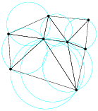
A Delaunay triangulation D of V is a simplicial complex such that all simplices are Delaunay, and the underlying space of D is the convex hull of V [6]. Figure 1 left illustrates a 2d Delaunay triangulation. A 3d Delaunay triangulation is also called a Delaunay tetrahedralization.
A Delaunay triangulation of V is unique if V is in general position, i.e., no d+2 points in V lie on a common sphere. Otherwise, we say that V contains degeneracies, i.e., there are d+2 points in V lie on a common sphere. Degeneracies can be removed by applying an arbitrary small perturbation onto the coordinates of points in V.
The dual of the Delaunay triangulation is the Voronoi diagram defined on the same vertex set (see Figure 1 right). For any vertex p ∈ V, the Voronoi cell of p is the set of points with distance to p not greater than to any other vertex of V, i.e. it is the set cell(p) = { x ∈ ℝd ; ||x − p|| ≤ ||x − q||, ∀ q ∈ V }, where || · || stands for the Euclidean distance. The Voronoi diagram of V is a subdivision of ℝd into Voronoi cells (some of which may be unbounded) and their faces [27]. It is a d-dimensional polyhedral complex. If the point set V is in general position, there is a one-to-one correspondence between the k-simplices of the Delaunay triangulation and the (d−k)-polyhedra of the Voronoi diagram, where 0 ≤ k ≤ d. In ℝ3, the vertices of the Voronoi diagram are the circumcenters of the tetrahedra of the Delaunay tetrahedralization.
There is a nice relation between a Delaunay triangulation in ℝd and a convex hull in ℝd+1. For any point p = (p0, p1, ⋯, pd−1) ∈ ℝd, define its lifted point p+ = (p0, p1, ⋯, pd−1, pd) ∈ ℝd + 1, where pd = p02 + ⋯ + pd−12. For any point set V ⊂ ℝd, define V+ = {p+ ; p ∈ V} ⊂ ℝd+1 be the lifted point set of V. All points in V+ lie on a paraboloid in ℝd + 1 (see Figure 2 left). The convex hull of V+ is a (d + 1)-dimensional convex polytope P. A lower face of P is a face of P which is on the downside of P (visible by points in V). The Delaunay triangulation of V is the projection of the set of lower faces of P onto d dimensions. Figure 2 right illustrates the relationship when d = 2. A simplex σ is a Delaunay simplex if and only if there exists a hyperplane in ℝd+1 passing through the lifted vertices of σ such that no other lifted vertices in V+ lies below of it. Similarly, the Voronoi diagram of V is the projection of the lower faces of a convex polytope Q ⊂ ℝd+1 such that P and Q are polar to each other [29].
Weighted Delaunay triangulations are generalizations of Delaunay triangulations by replacing the Euclidean distance by “weighted distance”.
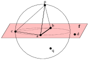
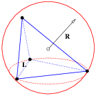
A weighted point, p′ = (p, p2) ∈ ℝd × ℝ, can be interpreted as a sphere centered at p with radius p. The weighted distance between p′ and z′ is
| πp′, z′ = | √ |
| , |
see Figure 3 left for an example. In particular, points in ℝd can be considered weighted points with zero weight.
Two weighted points p′, z′ are orthogonal if their weighted distance is zero, i.e.,
| ||p − z ||2 = (p2 + z2). |
We say that two weighted points are farther than orthogonal when their weighted distance is positive, and closer than orthogonal when the distance becomes an imaginary number.
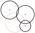
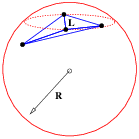
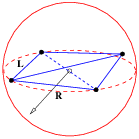
In general, d+1 points in ℝd define a unique circumsphere passing through them. Similarly, d+1 weighted points in ℝd define a unique common orthosphere. When all points have zero weights, their orthosphere is just their circumsphere. Figure 3 (right) gives an example of the orthosphere of three weighted points in two dimensions.
Let V′ ⊂ ℝd × ℝ be a finite set of weighted points. We say a sphere is empty if all weighted points in V′ are farther than orthogonal of it. The weighted Delaunay triangulation of V′ is a simplicial complex D′ such that every simplex has an orthosphere which is empty, and the underlying space of D′ is the convex hull of V′. Obviously, if all the points have the same weight, the weighted Delaunay triangulation is the same as the usual Delaunay triangulation. Note that, a weighted Delaunay triangulation does not necessarily contain all points in V′.
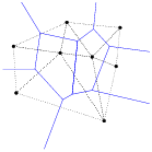
The dual of a weighted Delaunay triangulation is a weighted Voronoi diagram, also called the power diagram [1, 9] of the weighted point set V′. Power diagrams can be similarly defined as the Voronoi diagram by using the weighted distance instead of the Euclidean distance. If no d + 2 weighted points of V′ share a common orthosphere, i.e., it is in general position, then the simplices of the weighted Delaunay triangulation and the cells of the power diagram have a one-to-one correspondence. In ℝ3, the vertices of the power diagram are the orthocenters of the tetrahedra of the weighted Delaunay tetrahedralization.
A weighted Delaunay triangulation of V ⊂ ℝd is also the projection of the set of lower faces of a convex polytope P ⊂ ℝd+1. Any point in p = {p0, ..., pd−1} ∈ V is lifted to a point p′ = {p0, ..., pd−1, pd} ∈ ℝd+1, where pd = p02 + ⋯ + pd−12 − p2 (p is the weight of p). For p ≠ 0, p′ does not lie on a paraboloid in ℝd+1, but is moved vertically downward by p2. A simplex belongs to the weighted Delaunay triangulation of V (i.e., it has an empty orthosphere) if and only if there exits a hyperplane passing through the lifted weighted points of these simplex and no lifted weighted point of V lie below the hyperplane.
Both weighted Delaunay triangulations and power diagrams are called regular subdivisions of point sets [29]. Regular subdivisions have nice combinatorial structures. They are one of the important objects studied in higher-dimensional convex polytopes [29, 5].
Algorithms for generating Delaunay (and weighted Delaunay) tetrahedralizations are well studied in computational geometry [7]. TetGen implemented two algorithms, the Bowyer-Watson algorithm [3, 28] and the incremental flip algorithm [9]. Both algorithms are incremental, i.e., insert points one after another. Both have the worst case runtime O(n2). In most of the practical applications, they are usually very fast. The expected running time of these algorithms is O(n logn) if the points are uniformly distributed in [0,1]3.
The speed of incremental algorithms is very much affected by the cost of point location. TetGen uses a spatial sorting scheme [2] to improve the point location. The idea is to sort the points such that nearby points in space have nearby indices. The points are first randomly sorted in different groups, then points in each group are sorted along the Hilbert curve. Inserting points in this order, each point location can be done in nearly constant time.
TetGen uses Shewchuk’s exact geometric predicates [15] for performing the Orient3D, InSphere, and Orient4D tests. These suffice to guarantee the numerical robustness of generating Delaunay and weighted Delaunay tetrahedralizations. A simplified symbolic perturbation scheme [8] is used to remove the degeneracies.
A tetrahedral mesh is a 3d simplicial complex that is a discrete representation of a 3d continuous space (domain), both in its topology and geometry. Note that a Delaunay tetrahedralization is a tetrahedral mesh of the convex hull of its vertex set. In general, a geometric domain may not be convex and may have arbitrarily complex boundaries.
The input domain of TetGen is modeled by a piecewise linear complex (Section 1.2.1). The focuses of TetGen are the representation of the geometry (the boundary) and the quality of the mesh. TetGen generates several types of tetrahedral meshes to achieve these goals. They are explained in the following subsections.
At first we need a model to represent a 3d domain such that it can be easily described and handled. A 3d piecewise linear complex (PLC) X is a set of cells, that satisfies the following properties:
It is first introduced by Miller, et al. [11], see Figure 4 left for an example.

A 3d PLC non-PLCs
Figure 4: Left: A 3d piecewise linear complex. The left shaded area shows a facet, which is non-convex and has a hole in it. It has also edges and vertices floating in it. The right shaded area shows an interior facet separating two sub-domains. Right: Configurations which are not PLCs.
The boundary of a 3d PLC is the set of cells whose dimensions are less than or equal to 2. A 0-dimensional cell is a vertex. In particular, we call a 1-dimensional cell (an edge) a segment, and a 2-dimensional cell a facet. Each facet of a PLC is a 2d PLC. It may contain holes, segments and vertices in its interior, see Figure 4 left for an example.
PLCs are flexible in describing 3d geometric features. For instance, they permit facets, segments and vertices to float in a domain, or segments and vertices to float in the facet. One purpose of these floating cells is to constrain how the PLC can be meshed, so that boundary conditions may be applied at those cells.
The definition of a PLC disallows illegal intersections of its cells, see Figure 4 right for examples. Two
segments only can intersect at a common vertex that is also in
X. Two facets of X may intersect only at a union of vertices and segments which are also in X.
The underlying space of a PLC X,
denoted | X|, is ∪f ∈ X f,
which is the domain to be triangulated.
A tetrahedral mesh of X,
is a 3d simplicial complex T such that
(1) X and T have the same vertices,
(2) every cell in X is a union of simplices in T, and
(3) | T| = | X|.
Let T be a tetrahedral mesh of a 3d PLC X. The boundary of X is respected by the elements of T, i.e., each segment of X is represented by a union of edges in T, and each facet of X is represented a union of triangles in T.
To distinguish those edges and triangles of T which are on segments and facets of X, we call them boundary edges and boundary faces.
TetGen uses a simple boundary representation (a surface mesh) to represent a 3d PLC. It is explained in Section 5.1.1 and in the file formats .poly and .smesh of TetGen.
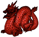
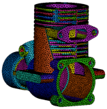
Figure 5 shows two typical surface meshes of 3d PLCs. The following points are useful to know.
A PLC only gives a piecewise linear approximation of a 3d domain. It does not take the curvature of the surfaces into account. When TetGen modifies the surface mesh, it only modifies the linear edges and facets. This is unfortunately a limitation of using PLC.
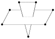
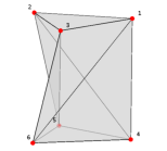
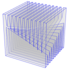
There are 3d polyhedra which may not be tetrahedralized with only its own vertices, two typical examples are shown in Figure 6. Nevertheless, it is always possible to tetrahedralize a polyhedron if Steiner points (which are not vertices of the polyhedron) are allowed.
A Steiner tetrahedralization of a PLC X is a tetrahedralization of X ∪ S, where S is a finite set of Steiner points (disjoint from the vertices of X). TetGen generates Steiner tetrahedralizations of PLCs. Two types of Steiner points are used in TetGen:
In both cases, TetGen tries to generate the Steiner points efficiently and limit the number of Steiner points as small as possible. The optimal locations and the optimal number of Steiner points is still a topic of research.
A fundamental problem in mesh generation is how to enforce a set of constraints, such as edges and triangles, to be preserved or represented by a mesh. These constraints usually describe the special features in the domain boundaries, such as the boundary complex of a PLC, and they are required to be correctly represented in the generated meshes. It is generally referred to the boundary conformity or boundary recovery problem.
Boundary conformity in 2d is very easy. One can enforce any edge (which does not intersect any boundary) into a triangulation. Moreover, it does not need any Steiner point. However, it is very difficult in 3d since it is not always possible to enforce an edge or a triangle into a tetrahedralization without using Steiner points.
TetGen always respects the boundary of the domain. TetGen can generate different types of (Steiner) tetrahedralizations such that input segments and facets of a PLC are respected.
These different types of tetrahedralizations produced by TetGen may find use in different situations. For instances, conforming DTs are desired for applications which need the Delaunay property. While this type of tetrahedralization usually need a large number of Steiner points. CDTs require much less Steiner points. They are an alternative choice of conforming DTs when the applications can accept non-Delaunay elements. Constrained tetrahedralizations are useful in many engineering applications for which the input domain boundaries need to be preserved.
A constrained Delaunay tetrahedralization (CDT) is a variation of a Delaunay tetrahedralization that is constrained to respect the edges and facets of X. CDTs in the plane were introduced by Lee and Lin [10]. Shewchuk [16, 21] generalized them into three or higher dimensions.
In the following, we give two equivalent definitions of constrained Delaunay tetrahedralizations.
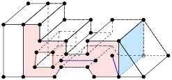
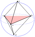
The visibility between two vertices p, q ∈ | X| is called occluded if there is a facet f ∈ X such that p and q lie on opposite sides of the plane that includes f, and the line segment pq intersects this facet (see Figure 7). A tetrahedron t whose vertices are in X is constrained Delaunay if its circumsphere encloses no vertex of X, which is visible from any point in the relative interior of t (see Figure 7 Left).
A tetrahedralization T is a constrained Delaunay tetrahedralization of X if it is a tetrahedralization of X and every tetrahedron of T is constrained Delaunay.
Let s be a triangle in a tetrahedralization T of X. s is said to be locally Delaunay if either it belongs to only one tetrahedron of T, or it is a face of exactly two tetrahedra t1 and t2 and it has a circumsphere which does not enclose any vertex of t1 and t2. Equivalently, the circumsphere of t1 encloses no vertex of t2 and vice versa (see Figure 7 Right). A tetrahedralization T of P is a CDT of P if every triangle in T not included in any facet of P is locally Delaunay.
The definitions of Delaunay tetrahedralization and constrained Delaunay tetrahedralization are almost the same except that, for the CDT, we free the requirement of being locally Delaunay for triangles in the facet. Hence CDTs retain many nice properties of those of Delaunay tetrahedralizations, see [21, 23]. Note that simplices (tetrahedra, triangles, and edges) in a CDT are not always Delaunay.
A CDT of an arbitrary PLC X may not exist [21]. Steiner points are necessary to ensure the existence of a CDT. A Steiner CDT of X is a CDT of X ∪ S, where S ⊂ | X| is a set of Steiner points.
Compared to conforming Delaunay tetrahedralizations, (Steiner) CDTs usually require much less Steiner points.
There is no unique definition of the term “mesh quality". It depends on the intended application and the numerical methods employed, see, e.g. [19].
As a general guideline, elements with very small and large angles (and dihedral angels) should be avoided since they usually downgrade the accuracy and performance of numerical methods.
Figure 8 shows six differently shaped tetrahedra. A tetrahedron shape measure is a continuous function which evaluates the shape of a tetrahedron by a real number. Various tetrahedron shape measures have been suggested, some of them are equivalent.
The most general shape measure for a simplex is the aspect ratio. The aspect ratio, η(τ), of a tetrahedron τ is the ratio between the longest edge length lmax and the shortest height hmin, i.e., η(τ) = lmax/hmin. The aspect ratio measures the “roundness" of a tetrahedron in terms of a value between √2/√3 and +∞. A low aspect ratio implies a better shape. Other possible definitions of aspect ratio exist, such as the ratio between the circumradius and inradius. These definitions are equivalent in the sense that if a tetrahedralization is bounded w.r.t. one of the ratios then it is bounded w.r.t. all the others.
The tetrahedron shape measures used in TetGen are the face angles (angles between two edges) and dihedral angles (angles between two faces) as the shape measures of tetrahedra. They work well with the Delaunay refinement algorithm used in TetGen. Also, the combination of them achieve the same objective as the aspect ratio.
To bound the smallest face angle is equivalent to bound the radius-edge ratio of the tetrahedron. The radius-edge ratio, ρ(τ) of a tetrahedron τ is the ratio between the radius r of its circumscribed ball and the length d of its shortest edge, i.e.,
| ρ(τ) = |
| ≥ |
| , |
where θmin is the smallest face angle of τ, see Figure 9. The radius-edge ratio ρ(τ) is at least √6/4 ≈ 0.612, achieved by the regular tetrahedron. Most of the badly shaped tetrahedra will have a big radius-edge ratio (e.g., > 2.0) except the sliver, which is a type of very flat tetrahedra having no small edges, but nearly zero volume. A sliver can have a minimal value √2/2 ≈ 0.707, hence the radius-edge ratio is not equivalent to aspect ratio (due to the slivers). Nevertheless, the radius-edge ratio is a useful shape measure. It can be shown that if a tetrahedral mesh has a radius-edge ratio bounded for all of its tetrahedra, then the point set of the mesh is well spaced, and each node of the mesh has bounded degree [11, 23].
Each of the six edges of a tetrahedron τ is surrounded by two faces. At a given edge, the dihedral angle between two faces is the angle between the intersection of these faces and a plane perpendicular to the edge. The dihedral angle in τ is between 0∘ and 180∘. The minimum dihedral angle φmin(τ) of τ is a tetrahedron shape measure used by TetGen.
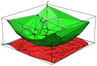
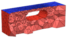
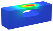
The goal of adaptive mesh generation is to generate a mesh which achieves the desired mesh quality with a small number of mesh elements. In numerical methods, such a mesh gives a good balance between the solution time and the accuracy of the solution, see Figure 10 for an example.
The total number of mesh element is determined by the mesh element sizes, i.e., the diameters of the mesh elements. It is in general no possible to determine a proper mesh element size in advance. It depends on the actual applications and the numerical methods employed.
As a general guideline for adaptive mesh generation, TetGen uses a mesh sizing function. Let X be a 3d PLC. A mesh sizing function H: | X| → ℝ, is a function that maps each point p ∈ | X| to a positive value H(p) which specifies the desired mesh edge lengths at the point location p. Typically, the mesh sizing function can be the geometrical features of the input PLC, an error distribution function obtained from a previous numerical solution, or a user-specified function.
A mesh sizing function H is isotropic if the edge length does not vary with respect to the directions at p, otherwise, it is anisotropic. The current version of TetGen only supports isotropic mesh sizing functions. An ideal sizing function is C∞, ∀ p ∈ | X|. However, in most cases, H is approximated by a discrete function specified at some points in | X|. The size at other points in | X| is obtained by means of interpolation.
TetGen supports several ways of defining a sizing function. It can be defined automatically, explicitly on various sources of volumes, facets, line segments, and points, or through user-defined sizing functions.
All the above ways of defining sizing function can be used at the same time. TetGen will automatically choose the smallest mesh element size. In the last two ways, i.e., defining mesh element sizes on nodes, it is possible to set the size to zero at a node. In this case, the mesh element size at this location is ignored.
Mesh optimization is an essential way for further improving the mesh quality. Typically, it improves one or several objective functions on mesh quality, such as the aspect ratio, minimum or maximum dihedral angles, etc.
Mesh optimization is usually done by applying various local mesh operations which either change the node locations or change the mesh connections. The most frequently used operations are: node smoothing, edge/face swapping, edge contraction, and vertex insertion. These operations are combined according to a schedule to iteratively improve the mesh quality. One can decide to either optimize the whole mesh (global optimization) or only optimize a part of the mesh (local optimization).
TetGen uses mesh optimization after the mesh generation. It locally optimizes the tetrahedral mesh to restore the Delaunay property and to improve the mesh quality. The current version uses the maximum dihedral angle as objective function. It provides options to choose local operations and to restrict the maximum number of iterations in the optimization procedure, see the -O switch.
Algorithms for constructing 3d CDTs were first considered by Shewchuk. In [16], a sufficient condition for the existence of a CDT of a PLC (or a polyhedron) is given. Based on this condition, several algorithms for constructing Steiner CDTs are proposed [18, 20, 26, 25]. TetGen’s CDT algorithm is from Si and Gärtner [26, 25].
The basic algorithm for generating quality tetrahedral meshes is the Delaunay refinement algorithm from Ruppert [13] and Shewchuk [17]. This algorithm generates a quality mesh of Delaunay tetrahedra with no tetrahedra having a radius-edge ratio greater than 2.0 (equivalently, no face angle less than 14.5o). The sizes of tetrahedra are graded from small to large over a short distance. TetGen implemented this algorithm for improving the mesh quality of a CDT of a PLC. In practice, the algorithm generates meshes generally surpassing the theoretical bounds and eliminates tetrahedra with small or large dihedral angles efficiently.
There are two theoretical problems of the basic Delaunay refinement algorithm. First, it does not remove slivers due to the use of radius-edge ratio as the sole tetrahedral shape measure. Second, it may not terminate if the input PLC X contains sharp features, i.e., there are two edges of X meeting at an acute angle, or two facets of X meeting at an acute dihedral angle.
TetGen uses the minimal dihedral angle of tetrahedron as a second shape measure for the Delaunay refinement algorithm, hence slivers are found by this measure and are removed by the above mentioned Delaunay refinement iterations. Since TetGen works with CDTs, it can detect all the sharp features in the CDT in advance. Then it starts the Delaunay refinement process. Tetrahedra at the sharp features are never removed. The modified algorithm in TetGen always terminates. However some badly-shaped tetrahedra near the sharp features may survive.
TetGen accepts a user-defined mesh sizing function to control the mesh element size. If this is given, TetGen will generate an adaptive tetrahedral mesh according to the input mesh sizing function. It uses a constrained Delaunay refinement algorithm [22].
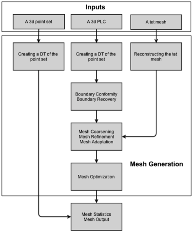
Figure 11 shows a graphic flowchart of the meshing process in TetGen.
Here are the general steps of TetGen to create a (quality) tetrahedral mesh. Many of these steps can be skipped, depending on the command line switches.